The povray module

All figures in this manual have been exported directly from the morpho programs that created them using the persistence of vision raytracer or povray. A raytracer is a program that takes a scene description and renders graphical output by tracing the path of individual rays of light. Because the model of light propagation and image formation is physically motivated, the output is of very high quality. By contrast, morphoview and most graphics programs use simplified approximate rendering techniques that enable real time interactive output. At the time of writing, raytracing is gaining popularity as a technique, and some high performance graphics cards now have real time raytracing capability. povray is a very well established program that is widely available and cross platform.

To use the povray module, you need to create a POVRaytracer object and initialize it with the graphics object

import povray

var pov = POVRaytracer(g)

You can choose features of the graphics out by setting properties of this object, for example:

pov.viewpoint = Matrix([5,5,6]) // Sets where the camera is located
pov.viewangle = 18 // Controls the angular size of the view
pov.background = White // Sets the background for rendering
pov.light=[Matrix([10,10,10]), Matrix([0,0,10]), Matrix([-10,-10,10])] // Places light point sources at several positions

Because the list of properties can get quite cumbersome, it's possible to specify them through a separate Camera object and initialize the raytracer to use the Camera:

var pov = POVRaytracer(g, camera=cam)

See the Reference section for further details.

To produce output, call the render method to create a .pov file and run povray:

pov.render("graphic.pov")

By default, the resulting .png file is opened. You can stop this by calling render with display set to false:

pov.render("graphic.pov", display=false)

If you wish to simply create .pov file without running povray, use the write method:

pov.write("graphic.pov")

**Randomly generated spheres** rendered with random transparency.

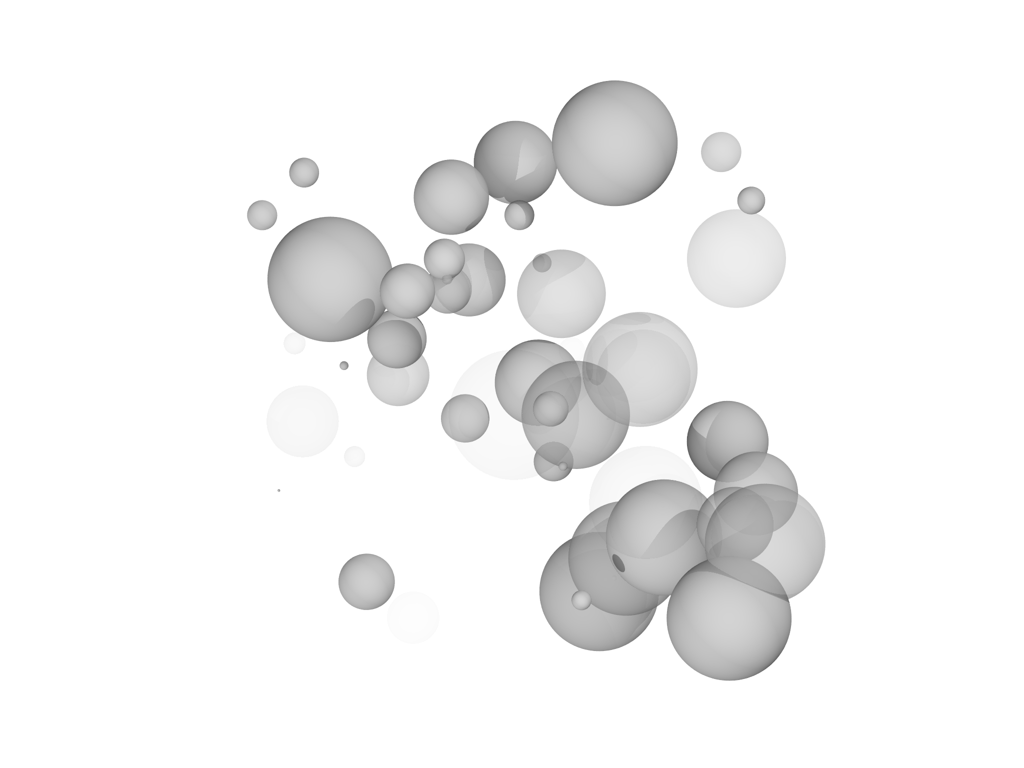
A major advantage of raytracing is natural support for transparency effects. Here we generate 50 spheres of random placement, size and transparency by setting the transmit option. The rendered output is shown in Fig. 6.7.

fn randompt(R) {
    return R*Matrix([random()-1/2, random()-1/2, random()-1/2])
}

for (i in 1..50) {
    g.display(Sphere(randompt(1.5), random()/5, transmit=random()))
}