Thomson
Consider \(N\) charges \(q\) with positions \(x_i\) that are each confined to lie on the unit sphere so that \(\left| x_i\right|=1 \) that repel each other electrostatically and hence whose configuration minimizes the energy, $$\frac{k}{2}\sum_{i\neq j}\frac{q^{2}}{\left|x_{i}-x_{j}\right|}$$ The problem was posed by the physicist J. J. Thomson in 1904, in the context of an early model for the structure of an atom.
To set this up in morpho, we begin by creating a mesh from a sequence
of random points using a MeshBuilder object from the meshtools module.
Notice that this is quite an unusual mesh; it consists of \(N\)
unconnected points with no connectivity information.
var build = MeshBuilder()
for (i in 1..Np) {
  var x = Matrix([2*random()-1, 2*random()-1, 2*random()-1])
  x/=x.norm() // Project onto unit sphere
  build.addvertex(x)
}
var mesh = build.build()
The optimization problem is then specified. We use the PairwisePotential
functional from the functionals module and supply the Coulomb
potential \(1/r\), together with its derivative \(-1/r^{2}\) as anonymous
functions:
var problem = OptimizationProblem(mesh)
var lv = PairwisePotential(fn (r) 1/r, fn (r) -1/r^2)
problem.addenergy(lv)
Constraining the particles to a sphere is implemented as a level set constraint: We use the ScalarPotential functional as a local constraint to ensure that each particle lies on the zero contour of the scalar function \(x^{2}+y^{2}+z^{2}-1\), which defines the unit sphere.
var lsph = ScalarPotential(fn (x,y,z) x^2+y^2+z^2-1) problem.addlocalconstraint(lsph)
Optimization is then performed:
var opt = ShapeOptimizer(problem, mesh)
opt.stepsize=0.01/sqrt(Np)
opt.relax(5)
opt.conjugategradient(1000)
Notice that we estimate the initial stepsize from the number of
particles. Since each particle will adopt a fraction \(1/N\) of the area,
the stepsize is \(\propto1/\sqrt{N}\). In practice, we find that taking a
few steps of gradient descent with relax helps condition the problem by
pushing any particles from the initially random distribution that
happened to be placed very close to one another apart. After this
conjugategradientworks well and typically converges in around \(100\)
iterations.
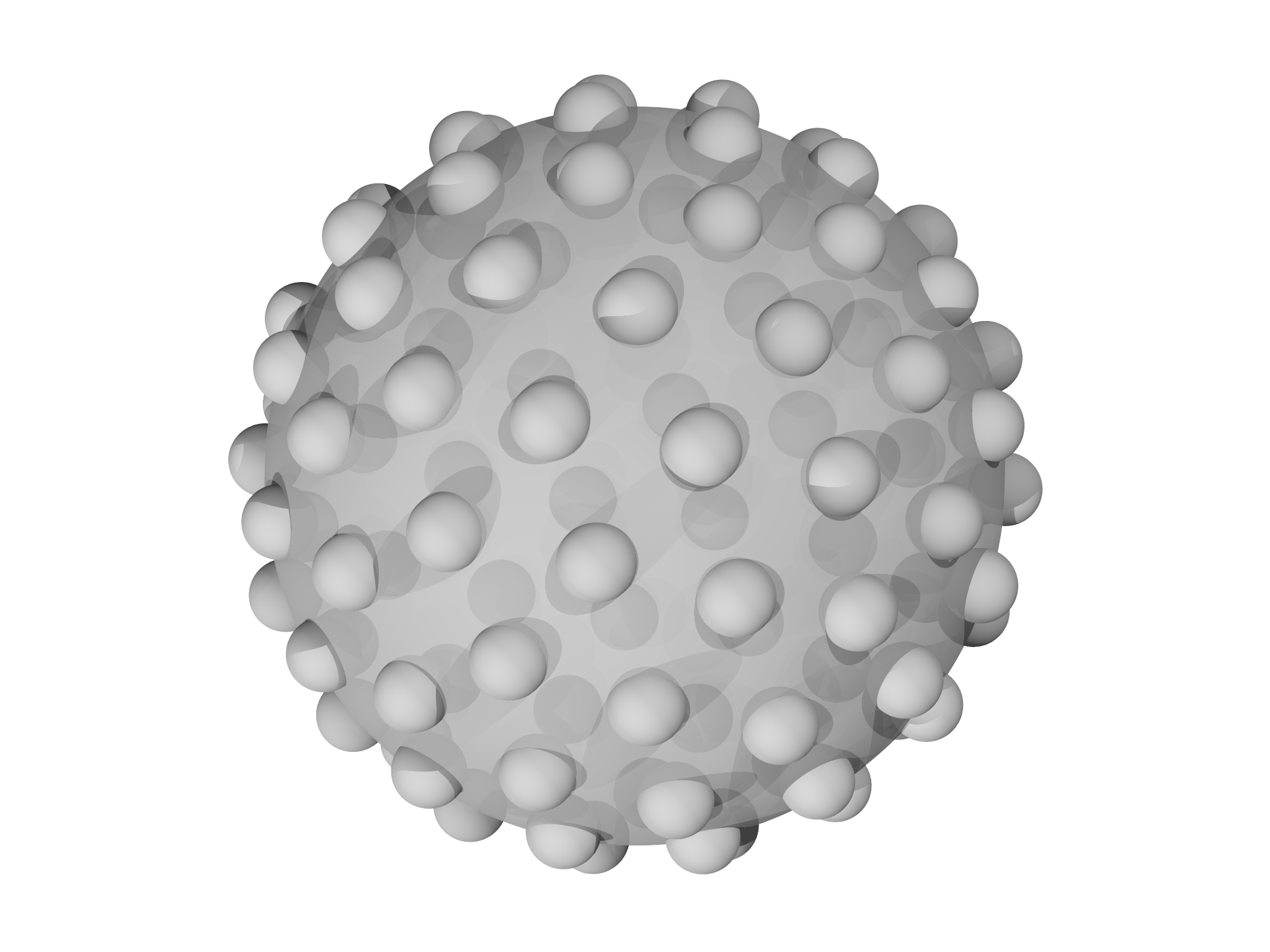
A final interesting feature of this example is the use of a custom visualization. We draw a sphere with a center of mass at the location at each particle:
var g = Graphics()
for (i in 0...mesh.count()) {
  g.display(Sphere(mesh.vertexposition(i),1/sqrt(Np)))
}
g.display(Sphere([0,0,0],1))
Show(g)
A typical configuration resulting from this is shown in Fig.
7.12. Note
that we made the large sphere transparent to render with the povray
module; this was achieved by adding the optional argument transmit=0.3
to the call to Sphere.