The graphics module
Support for low level graphics is provided by the graphics module,
which you can use this to create custom visualizations and generate
other kinds of graphical output. These can be easily combined with
output from the plot module, which utilizes graphics internally.
We begin by creating a Graphics object, which represents a scene or a collection of things to be displayed.
var g = Graphics()
Once the Graphics object is created, we can add display elements, objects specifying what is to be drawn, to the scene in turn.
Sometimes referred to as graphics 'primitives'.
The graphics module supports the following kinds of element:
-
Cylinder specified by two points at each end of the cylinder on its axis. You can also specify the aspect ratio, i.e. the ratio of the radius of the cylinder to its length, and the number of points to draw.
Cylinder([-1/2,-1/2,-1/2], [1/2,1/2,1/2], aspectratio=0.2, n=10) -
Arrow specified in the same way as a Cylinder, e.g.
Arrow([-1/2,-1/2,-1/2], [1/2,1/2,1/2], aspectratio=0.2, n=10) -
Sphere specified by the center and the radius, e.g.
Sphere([0,0,0], 0.8) -
Text specified by the text to display and the location to display at. Many options can be provided, including the drawing direction and the vertical direction, the size in points (1 graphics unit=72 points), and the Font.
Text("Hello World!", [-0.75,0,0], size=24, color=Black) -
Tube specified by a sequence of points and a radius. You can also specify if the tube is closed or not.
var pts = [] for (phi in -Pi..Pi:Pi/32) { pts.append([0.5*(1+0.3*sin(4*phi))*cos(phi), 0.5*(1+0.3*sin(4*phi))*sin(phi), 0]) } g.display(Tube(pts, 0.05, color=Blue, closed=true)) -
TriangleComplex describes a collection of triangles, which can be used to display polyhedra and other complex objects. These elements are low-level, and further information is available in the reference section.
Most of these elements accept certain optional arguments:
-
color to specify the color.
-
transmit specifies the transparency of the element, which by default is 0.
-
filter alternative way of specifying transparency for use with the povray module.
Once appropriate elements have been created, we can display the Graphics
object with morphoview using Show.
Show(g)
A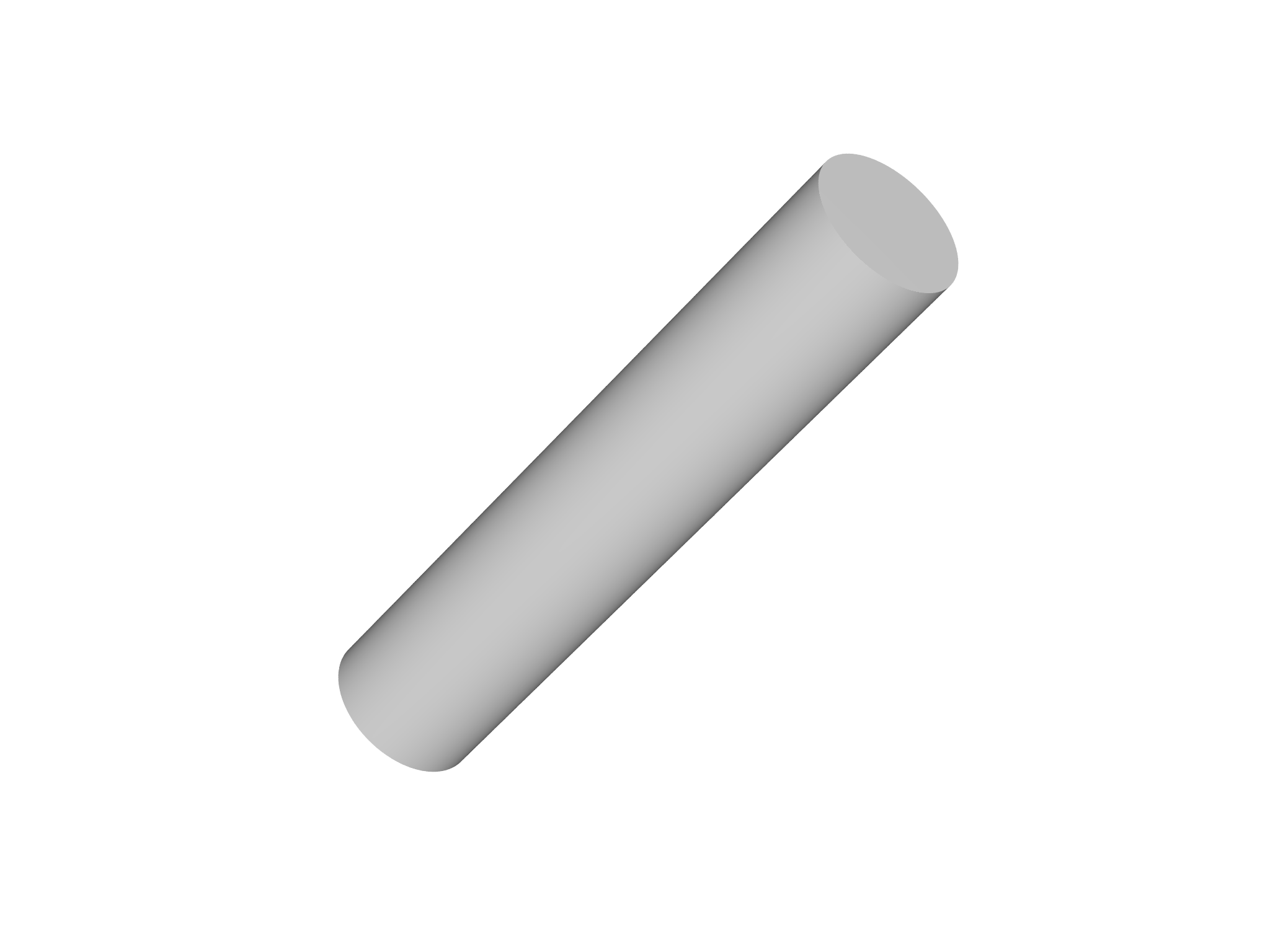 B
B![]() C
C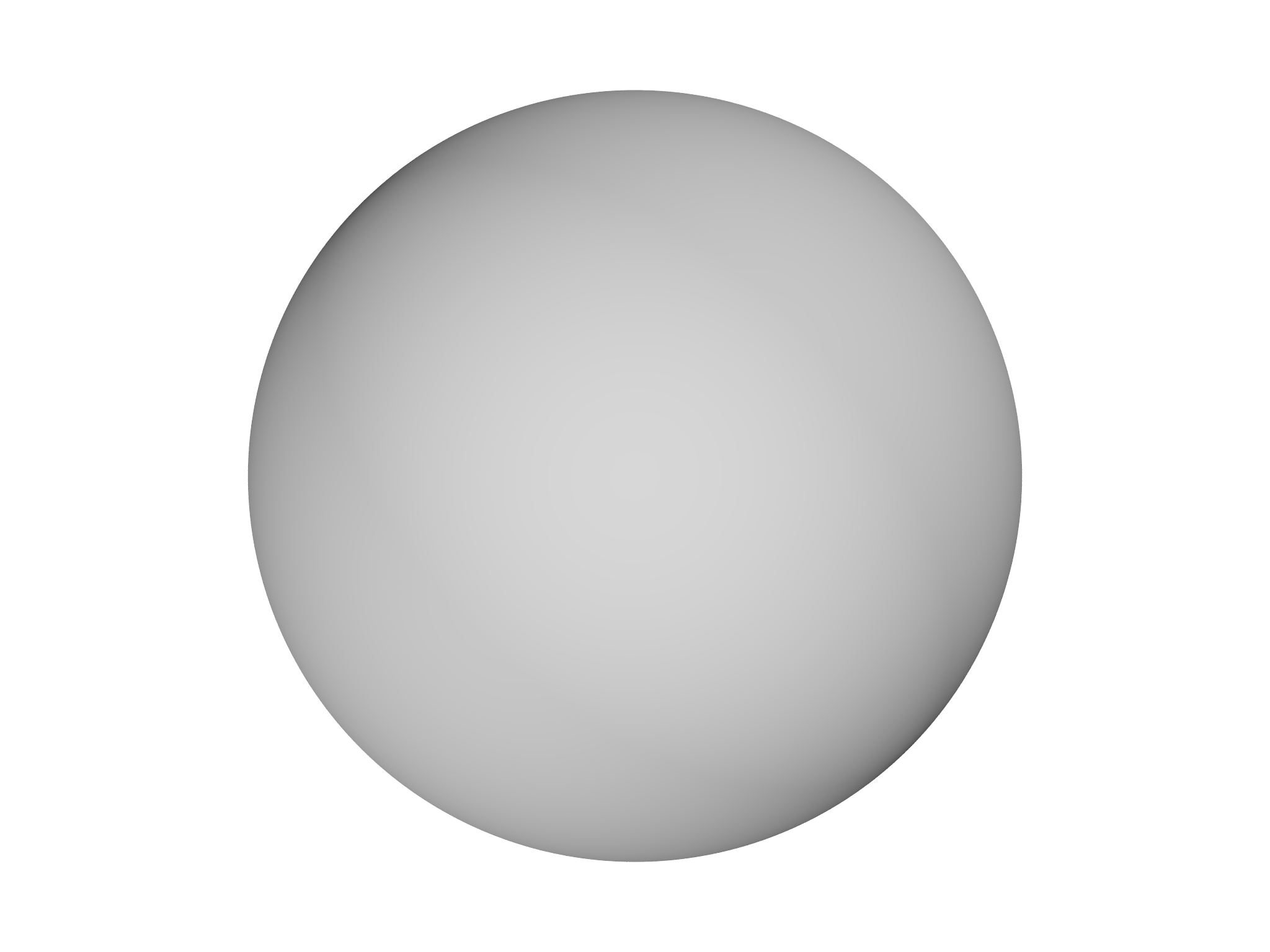
D E
E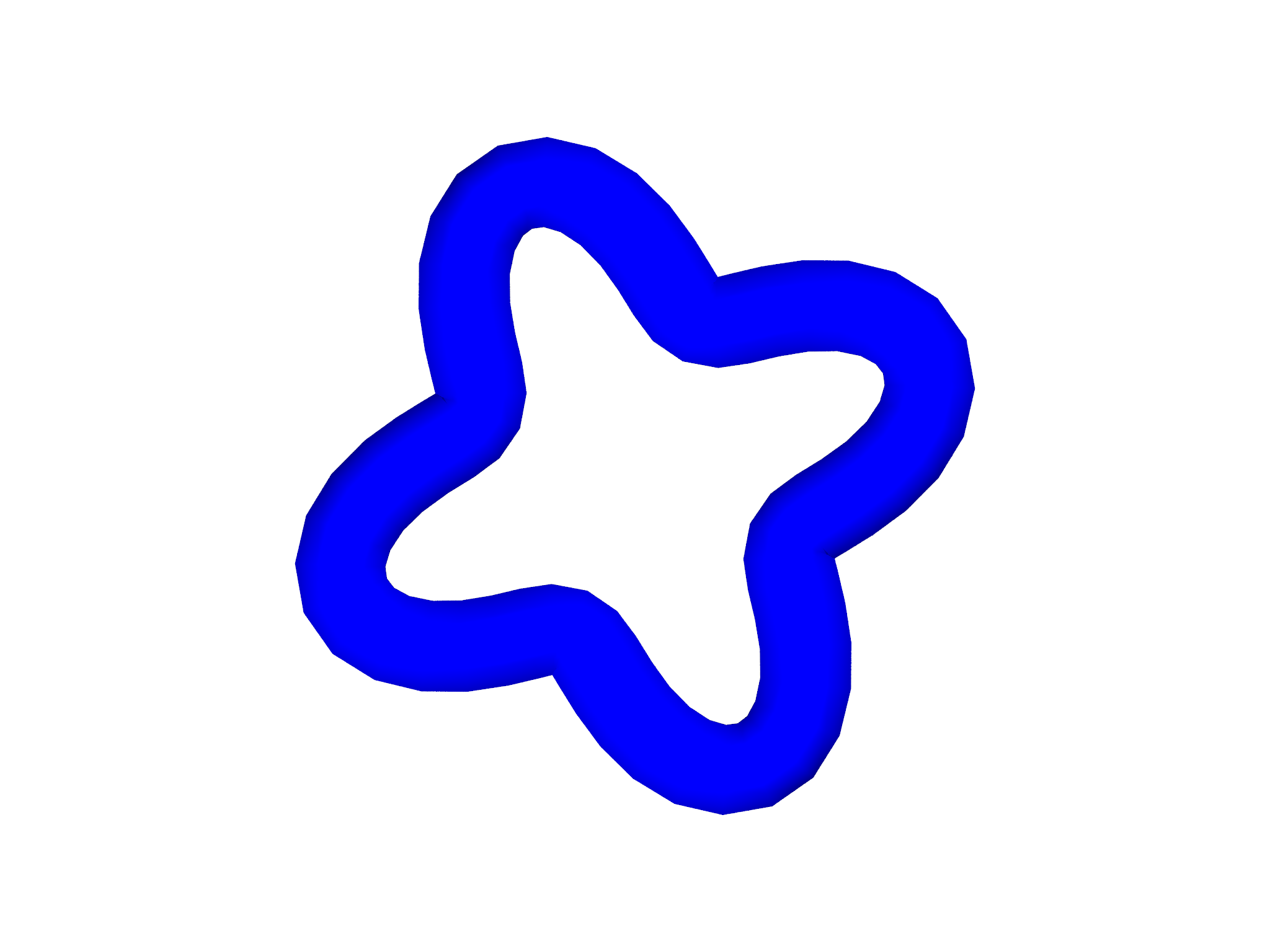 F
F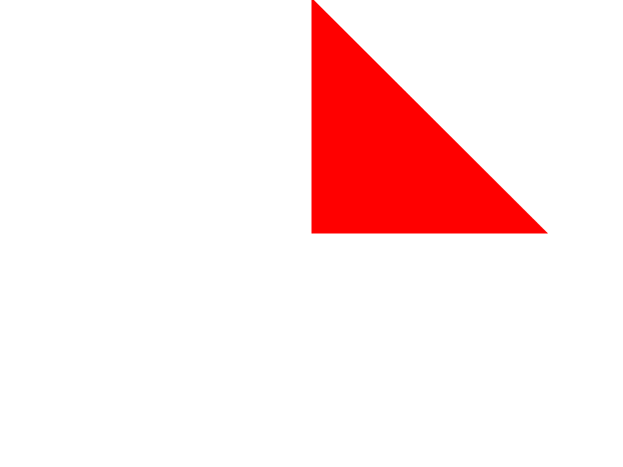
Example: Visualizing an electric field

As an illustration of what's possible using the graphics module
directly, we'll create a visualization of the electric field due to two
point charges (Fig. 6.6{reference-type="ref"
reference="fig:ElectricField"}). Begin by setting some constants and
creating the Graphics object:
var L = 2 // Size of domain to draw
var R = 1 // Separation of the charges
var dx = 0.125 // Spacing of points to draw
var eps = 1e-10 // Check for zero separation

var g = Graphics()
We'll now define the charges by creating two List objects: one contains the strength of each charge and the second stores their positions:
// Electric field due to a system of point charges
var qq = [1,-1]
var xq = [ Matrix([-R/2, 0, 0]), Matrix([R/2, 0, 0])]
We'll also define a cutoff distance around each charge below which we won't draw the electric field (remember it grows \(\to\infty\) as we get closer!):
var cutoff = 0.2
Next, we need a function that calculates the electric field at an arbitary point. We do this by summing up the electric fields due to each charge using Coulomb's law:
fn efield(x) {
   var e = 0
   for (q, k in qq) {
    var r=x-xq[k]
    if (r.norm()<cutoff) return nil
    e+=q*r/(r.norm()^3) // = 1/r^2 * \hat{r}
  }
  return e
 }
To draw the electric field, we create a rectangular grid of points, calculate the electric field at each point and draw an Arrow along the orientation.
var lambda = dx/10
for (x in -L..L:dx) for (y in -L..L:dx) {
  var x0 = Matrix([x,y,0])
  var E = efield(x0)
  if (isnil(E)) continue
  if (E.norm()>eps) g.display(Arrow(x0-lambda*E,x0+lambda*E))
}
We now draw the charges, coloring them by their sign:
for (q,k in qq) {
  var col = Red
  if (q<0) col = Blue
  g.display(Sphere(xq[k],dx/4,color=col))
}
Finally, we display the scene:
Show(g)