
Version 0.6.0
In nova fert animus mutatas dicere formas
corpora; di, coeptis (nam vos mutastis et illas)
adspirate meis primaque ab origine mundi
ad mea perpetuum deducite tempora carmen!
--- Ovid, Metamorphoses
Acknowledgements
The principal architect of morpho, T J Atherton, wishes to thank the many people who have used various versions of the program or otherwise contributed to the project:
| Andrew DeBenedictis | Danny Goldstein |
| Ian Hunter | Chaitanya Joshi |
| Cole Wennerholm | Eoghan Downey |
| Allison Culbert | Abigail Wilson |
| Zhaoyu Xie | Matthew Peterson |
| Chris Burke | Badel Mbanga |
| Anca Andrei | Mathew Giso |
| Sam Hocking | Emmett Hamilton |
| Hudson Ramirez | Paco Navarro |
| Emmanuel Flores |
This material is based upon work supported by the National Science Foundation under grants DMR-1654283 and OAC-2003820.
Overview
Morpho aims to solve the following class of problems. Consider a functional, $$F=\int_{C}f(q,\nabla q,\nabla^{2}q,...)d^{n}x+\int_{\partial C}g(q,\nabla q,\nabla^{2}q,...)d^{n-1}x,$$ where \(q\) represents a set of fields defined on a manifold \(C\) that could include scalar, vector, tensor or other quantities and their derivatives \(\nabla^{n}q\). The functional includes terms in the bulk and on the boundary \(\partial C\) and might also include geometric properties of the manifold such as local curvatures. This functional is to be minimized from an initial guess \( \{ C_{0},q_{0} \}\) with respect to the fields \(q\) and the shape of the manifold \(C\). Global and local constraints may be imposed both on \(C\) and \(q\).
Morpho is an object-oriented environment: all components of the problem, including the computational domain, fields, functionals etc. are all represented as objects that interact with one another. Much of the effort in writing a morpho program involves creating and manipulating these objects. The environment is flexible, modular, and users can easily create new kinds of object, or entirely change how morpho works.
This manual aims to help users to learn to use morpho. It provides installation instructions in Chapter 2, information about how to run the program in Chapter 3. A detailed tutorial is provided in Chapter 4, showing how to set up and solve an example problem. Chapter 5 provides information about working with meshes and Chapter 6 describes how to visualize the results of your calculation with morpho. The examples provided with morpho are described in Chapter 7. The remaining chapters, comprising the second part of the manual, provide a reference guide for all areas of morpho functionality.
Installing Morpho
Morpho is hosted on a publicly available github repository https://github.com/Morpho-lang/morpho. Morpho also requires two subsidiary programs, a terminal app hosted in https://github.com/Morpho-lang/morpho-cli, and a viewer application https://github.com/Morpho-lang/morpho-morphoview. Morpho is extendable, and packages providing additional functionality are hosted in git repositories.
For this release, morpho can be installed on all supported platforms using the homebrew package manager. Alternatively, the program can be installed from source as described below. We are continuously working on improving morpho installation, and hope to provide additional mechanisms for installation in upcoming releases.
Install with homebrew
The simplest way to install morpho is through the homebrew package manager. To do so:
-
If not already installed, install homebrew on your machine as described on the homebrew website.
-
Open a terminal and type:
brew update
brew tap morpho-lang/morpho
brew install morpho
If you need to uninstall morpho, simply open a terminal and type
brew uninstall morpho. It's very important to uninstall the homebrew
morpho in this way before attempting to install from source as below.
Install from source
The second way to install morpho is by compiling the source code directly. Morpho now leverages the CMake build system, which enables platform independent builds.
Where a morpho source installation puts things
A morpho installation includes help files, modules, and other resources. By default, these are installed in the /usr/local/ file structure as follows:
/usr/local/bin : The morpho and morphoview executables are placed here.
/usr/local/share/morpho : Help files and modules are stored here.
/usr/local/include/morpho : Morpho header files for building extensions.
/usr/local/lib/morpho : Morpho extensions.
Collect Dependencies
Morpho requires a few libraries to provide certain functionality:
blas/lapack : are used for dense linear algebra.
suitesparse : is used for sparse linear algebra.
See https://people.engr.tamu.edu/davis/suitesparse.html and publications for details
povray : is a ray-tracer that is used for publication-quality graphics (only
required by the povray module).
The terminal application uses
libgrapheme or,
libunistring: for unicode grapheme support.
Morphoview additionally requires
glfw : to provide gui functionality.
freetype : provides text display.
Each of these dependencies can be installed using any appropriate package manager.
-
Homebrew (preferred on macOS):
brew update brew install glfw suite-sparse freetype povray libgrapheme -
Apt (preferred on Ubuntu):
sudo apt update
sudo apt upgrade
sudo apt install build-essential
sudo apt install libglfw3-dev libsuitesparse-dev liblapacke-dev povray libfreetype6-dev libunistring-dev
Build the morpho shared library
The core piece of morpho is a shared library, that can then be used by multiple applications. To build it,
-
Obtain the source by cloning the github public repository:
git clone https://github.com/Morpho-lang/morpho.git -
Navigate to the
morphofolder and build the library:cd morpho mkdir build cd build cmake -DCMAKE_BUILD_TYPE=Release .. sudo make install -
Navigate back out of the morpho folder:
cd ../../
Build the morpho terminal app
The terminal app provides an interactive interface to morpho, and can also run morpho files.
-
Obtain the source by cloning the github public repository:
git clone https://github.com/Morpho-lang/morpho-cli.git -
Navigate to the
morpho-clifolder and build the library:cd morpho-cli mkdir build cd build cmake -DCMAKE_BUILD_TYPE=Release .. sudo make install -
Check it works by typing:
morpho6 -
Assuming that the morpho terminal app starts correctly, type
quitto return to the shell and thencd ../../to navigate back out of the morpho-cli folder.
Build the morphoview viewer application
Morphoview is a simple viewer application to visualize morpho results.
-
Obtain the source by cloning the github public repository:
git clone https://github.com/Morpho-lang/morpho-morphoview.git -
Navigate to the
morpho-clifolder and build the library:cd morpho-morphoview mkdir build cd build cmake -DCMAKE_BUILD_TYPE=Release .. sudo make install -
Check it works by typing:
morphoviewwhich should simply run and quit normally. You can then type
cd ../../to navigate back out of the morpho-morphoview folder.
Windows via Windows Subsystem for Linux (WSL)
Windows support is provided through Windows Subsystem for Linux (WSL), which is an environment that enables windows to run linux applications. We highly recommend using WSL2, which is the most recent version and provides better support for GUI applications; some instructions for WSL1 are provided below.
-
Begin by installing the Ubuntu App from the Microsoft store. Follow all the steps in this link to ensure that graphics are working.
-
Once the Ubuntu terminal is working in Windows, you can install morpho either through homebrew or by building from source.
Graphics On WSL1
If you instead are working on WSL1, then you need to follow these instructions to get graphics running. Unless mentioned otherwise, all the commands below are run in the Ubuntu terminal.
-
A window manager must be installed so that the WSL can create windows. On Windows, install VcXsrv. It shows up as XLaunch in the Windows start menu.
-
Open Xlaunch. Then,
-
choose 'Multiple windows', set display number to 0, and hit 'Next'
-
choose 'start no client' and hit 'Next'
-
Unselect 'native opengl' and hit 'Next'
-
Hit 'Finish'
-
-
In Ubuntu download a package containing a full suite of desktop utilities that allows for the use of windows.
sudo apt install ubuntu-desktop mesa-utilsTell ubuntu which display to use
export DISPLAY=localhost:0To set the DISPLAY variable on login type
echo export DISPLAY=localhost:0 >> ~/.bashrc[Note that this assumes you are using bash as your terminal; you will may to adjust this line for other terminals].
-
Test that the window system is working by running
glxgearswhich should open a window with some gears.
Updating morpho
As new versions of morpho are released, you will likely want to upgrade to the latest version. From the terminal:
-
If you used homebrew to install morpho, simply type,
brew upgrade morpho -
If you installed morpho manually, and still have the git repository folder on your computer, navigate to this with
cdand type,git pullwhich downloads any updates. You can then follow the above instructions to recompile morpho. It's not necessary to reinstall dependencies, but note that some new releases of morpho may require additional dependencies.
-
If you no longer have the original morpho git repository folder from which you installed morpho, simply rerun the installation from scratch as above. You shouldn't need to reinstall dependencies.
Uninstalling morpho
If you wish to uninstall morpho, you can do so simply from the terminal application.
-
If you used homebrew to install morpho, simply type
brew uninstall morpho -
Alternatively, if you built morpho from source, you can remove everything with
rm /usr/local/bin/morpho6
rm /usr/local/bin/morphoview
rm /usr/local/lib/libmorpho*
rm -r /usr/local/share/morpho
rm -r /usr/local/lib/morpho
You may need to prefix these with
sudo.
Using Morpho
Morpho is a command line application, like python or lua. It can
be used to run scripts or programs, which are generally given the
.morpho file extension, or run interactively responding to user
commands.
Running a program
To run a program, simply run morpho with the name of the file,
morpho6 script.morpho
Morpho supports a number of switches:
-w : Run morpho with more than one worker thread, e.g. -w 4 runs morpho with 4 threads.
-D: Display disassembly of the program without running it. [See developer guide]
-d : Debugging mode. Morpho will stop and enter the debugger whenever a @ is encountered in the source. [See developer guide]
-p : Profile the program execution. Useful to identify performance bottlenecks. [See developer guide]
Interactive mode
To use morpho interactively, simply load the Terminal application (or equivalent on your system) and type
morpho6
Command line interface for Morpho
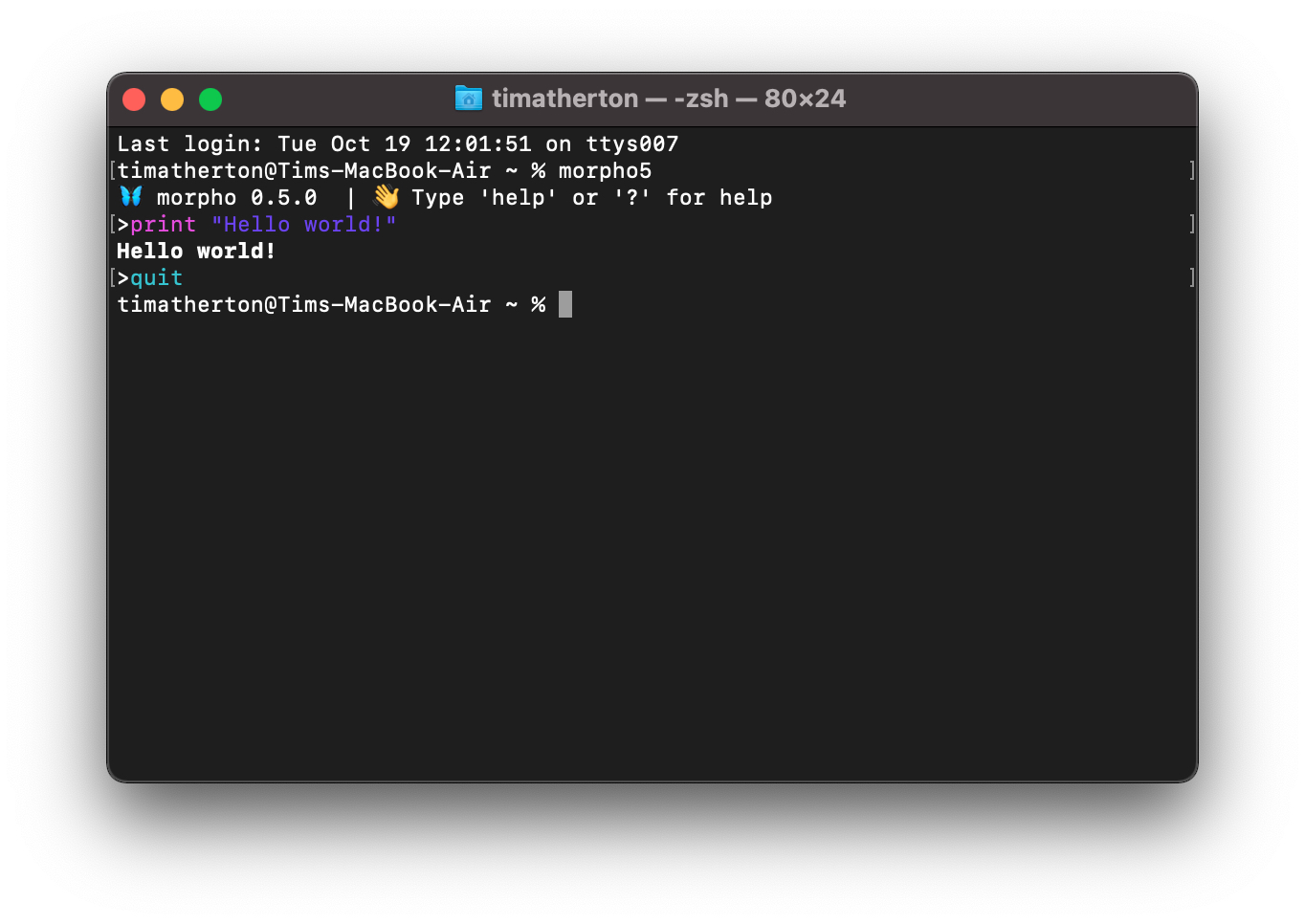
As shown in the figure above, you'll be greeted by a brief welcome and a
prompt > inviting you to enter morpho commands. For now, try a
classic:
print "Hello World"
which will display Hello World as output. More information about the
morpho language is provided in the Reference section, especially
chapter Language if you're familiar with C-like languages
such as C, C++, Java, Javascript, etc. things should be quite familiar.
To assist the user, the contents of the reference manual are available to the user in interactive mode as online help. To get help, simply type:
help
or even more briefly,
?
to see the list of main topics. To find help on a particular topic, for
example for loops, simply type the topic name afterwards:
? for
Once you're done using morpho, simply type
quit
to exit the program and return to the shell.
The interactive environment has a few other useful features to assist the user:
-
Autocomplete. As you type, morpho will show you any suggested commands that it thinks you're trying to enter. For example, if you type
vthe command line will show thevarkeyword. To accept the suggestion, press the tab key. Multiple suggestions may be available; use the up and down arrow keys to rotate through them. -
Command history. Use the arrow keys to retrieve previously entered commands. You may then edit them before running them.
-
Line editing. As you're typing a command, use the left and right arrows to move the cursor around; you can insert new characters at the cursor just by typing them or delete characters with the
deletekey. Hold down theshiftkey as you use the left and right arrow keys to select text; you can then useCtrl-Cto copy andCtrl-Vto paste.Ctrl-Amoves to the start of the line andCtrl-Ethe end.
Tutorial
To illustrate how to use morpho, we will solve a problem involving nematic liquid crystals (NLCs), fluids composed of long, rigid molecules that possess a local average molecular orientation described by a unit vector field \(\mathbf{n}\). Droplets of NLC immersed in a host isotropic fluid such as water are called tactoids and, unlike droplets of, say, oil in water that form spheres, tactoids can adopt elongated shapes.
The functional to be minimized, the free energy of the system, is quite complex,
$$ \begin{equation} F= \underbrace{\frac{1}{2}\int_{C}K_{11}\left(\nabla\cdot\mathbf{n}\right)^{2}+K_{22}(\mathbf{n}\cdot\nabla\times\mathbf{n})^{2}+K_{33}\left|\mathbf{n}\times\nabla\times\mathbf{n}\right|^{2}dA}_\text{Liquid crystal elastic energy}\label{eq:free} \end{equation} $$
$$ \begin{equation*} \quad + \underbrace{ \sigma\int dl }_\text{s.t.} \end{equation*} $$
$$ \begin{equation*} \quad + \underbrace{\frac{W}{2}\int\left(\mathbf{n}\cdot\mathbf{t}\right)^{2}dl}_\text{anchoring} \end{equation*} $$
where the three terms include liquid crystal elasticity that drives elongation of the droplet, surface
tension (s.t.) that opposes lengthening of the boundary and an
anchoring term that imposes a preferred orientation at the boundary.
We need a local constraint, \(\mathbf{n}\cdot\mathbf{n}=1\), and will also
impose a constraint on the volume of the droplet. For simplicity, we'll
solve this problem in 2D. The complete code for this tutorial example is
contained in the examples/tactoid folder in the repository.
Importing modules
Morpho is a modular system and hence we typically begin our program by
telling morpho the modules we need so that they're available for us to
use. To do so, we use the import keyword followed by the name of the
module:
    import meshtools
    import optimize
    import plot
We can also use the import keyword to import additional program files
to assist in modularizing large programs. These are the modules we'll
use for this example:
| Module | Purpose |
|---|---|
meshtools | Utility code to create and refine meshes |
optimize | Perform optimization |
plot | Visualize results |
Morpho language
The morpho language is simple but expressive. If you're familiar with C-like languages (C, C++, Java, Javascript) you'll find it very natural. A much more detailed description is provided in Chapter Language, but a brief summary is provided in the above figure and we provide an overview of key ideas to help you follow the tutorial:
-
Comments. Any text after
//or surrounded by/``*and*``/is a comment and not processed by morpho:// This is a comment /* This too! */ -
Variables. To create a variable, use the
varkeyword; you can then assign and use the variable arbitrarily:var a = 1 print a -
Functions. Functions may take parameters, and you call them like this:
print sin(x)and declare them like this:
fn f(x,y) {
    return x^2+y^2
}
Some functions take optional arguments, which look like this:
var a = foo(quiet=true) -
Objects. Morpho is deeply object-oriented. Most things in morpho are represented as objects, which provide methods that you can use to control them. Objects are made by constructor functions that begin with a capital letter (and may take arguments):
var a = Object()Method calls then look like this:
a.foo() -
Collections. Morpho provides a number of collection typesall of which are objectsincluding Lists,
var a = [1,2,3]and Dictionaries:
var b = { "Massachusetts": "Boston", "California": "Sacramento" }and Ranges (often used in loops):
var a = 0..10:2 # all even numbers 0-10 inclusiveThere are many others, including Matrices, Sparse matrices, etc.
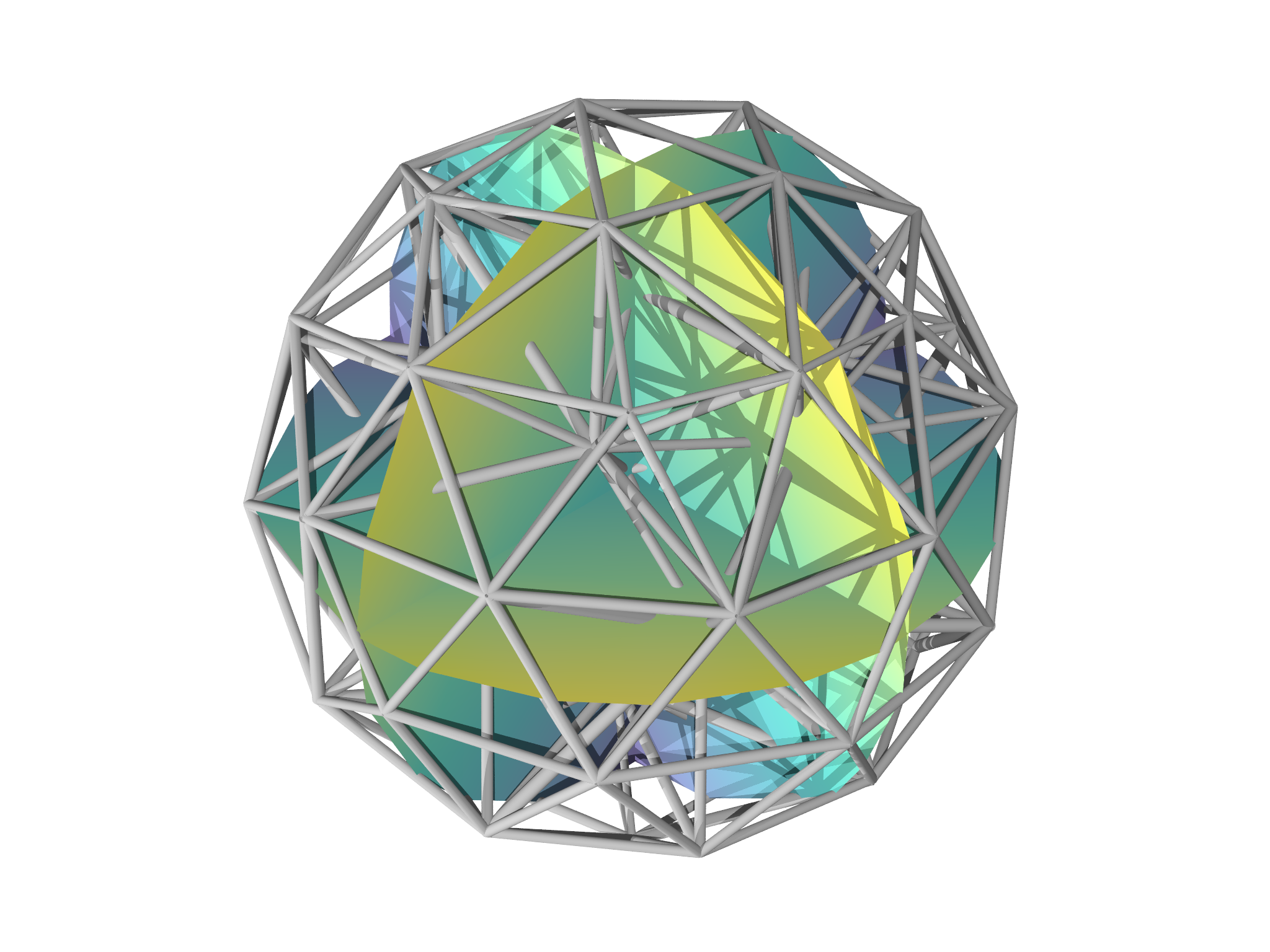
Creating the initial mesh

Meshes are discretized regions of space. The very simplest region we can
imagine is a point or vertex described by a set of coordinates
\((x_{1},x_{2},....,x_{D})\) where the number of coordinates \(D\) defines
the dimensionality of the space that the manifold is said to be
embedded in. From more than one point, we can start constructing more
complex regions. First, between two points we can imagine fixing an
imaginary ruler and drawing a straight line or edge between them.
Three points define a plane, and also a triangle; we can therefore
identify the two dimensional area of the plane bounded by the triangle
as a face, as in the face of a polyhedron. Using four points, we can
define the volume bounded by a tetrahedron. Each of these elements
has a different dimensionalitycalled a gradeand a complete Mesh may
contain elements of many different grades as shown in Fig.
4.2.
Morpho provides a number of ways of creating a mesh. One can load a mesh from a file, build one manually from a set of points, create one from a polyhedron, or from the level set (contours) of a function.
For this example, we'll use a predefined mesh file disk.mesh. To
create a Mesh object from this file, we call the Mesh function with
the file name:
var m = Mesh("disk.mesh")
Here, the var keyword tells morpho to create a new variable m, which now refers to the newly created Mesh object.
disk.mesh.The initial mesh is depicted in Fig. 4.3; we'll provide the code to perform the visualization in section Visualizing the results.
If you open the file disk.mesh, which you can find in the same folder
as tactoid.morpho, you'll find it has a simple human readable format:
vertices

1 -1. 0. 0
2 -0.951057 -0.309017 0
...

edges
1 8 2
2 2 4
...

faces
1 8 2 4
2 8 4 6
...
The file is broken into sections, each describing elements of a different grade. Each line begins either with a section delimiter such as vertices, edges or faces, or with an id. Vertices are then defined by a set of coordinates; edges and faces are defined by providing the respective vertex ids.
Selections
Sometimes, we want to refer to specific parts of a Mesh object:
elements that match some criterion, for example. Selection objects
enable us to do this. Because selecting the boundary is a very common
activity, the Selection constructor function takes an optional
argument to do this:
var bnd=Selection(m, boundary=true)
By default, only the boundary elements are included in the Selection.
For a mesh with at most grade 2 elements (facets), the boundaries are
grade 1 elements (lines); for a mesh with grade 3 elements (volumes),
the boundaries are grade 2 elements (facets). Quite often we want the
vertices themselves as well, so we can call a method to achieve that:
bnd.addgrade(0)
Once a Selection has been created, it can be helpful to visualize it
to ensure the correct elements are selected. We'll talk more about
visualization in section
Visualizing Results, but for now the line
Show(plotselection(m, bnd, grade=1))
shows a visualization of the mesh with the selected grade 1 elements shaded red as displayed in Fig. 4.4{reference-type="ref" reference="fig:Boundary"}.
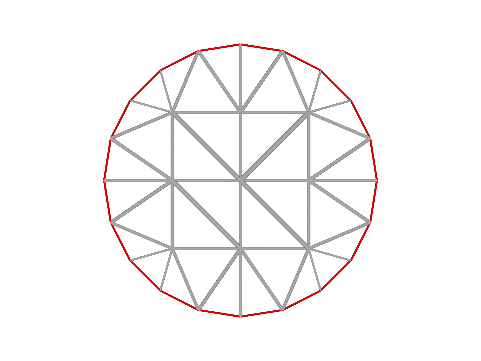 Selecting the boundary of the mesh
Fields
Having created our initial computational domain, we will now create a
Field object representing the director field \(\mathbf{n}\):
var nn = Field(m, Matrix([1,0,0]))
As with the Mesh object earlier, we declare a variable, nn, to refer
to the Field object. We have to provide two arguments to Field: the
Mesh object on which the Field is defined, and something to
initialize it. Here, we want the initial director to have a spatially
uniform value, so we can just provide Field a constant Matrix
object. By default, morpho stores a copy of this matrix on each vertex
in the mesh; Fields can however store information on elements of any
grade (and store both more than one quantity per grade and information
on multiple grades at the same time).
It's possible to initialize a Field with spatially varying values by
providing an anonymous function to Field like this:
var phi = Field(m, fn (x,y,z) x^2+y^2)
Here, phi is a scalar field that takes on the value \(x^{2}+y^{2}\). The fn keyword is used to define functions.
Defining the problem
We now turn to setting up the problem. Each term in the energy
functional (1) is represented by a corresponding functional
object, which acts on a Mesh (and possibly a Field) to calculate an
integral quantity such as an energy; Functional objects are also
responsible for calculating gradients of the energy with respect to
vertex positions and components of Fields.
Let's take the terms in (1) one by one: To represent the nematic elasticity we
create a Nematic object:
var lf=Nematic(nn)
The surface tension term involves the length of the boundary, so we need
a Length object:
var lt=Length()
The anchoring term doesn't have a simple built in object type, but we
can use a general LineIntegral object to achieve the correct result.
var la=LineIntegral(fn (x, n) n.inner(tangent())^2, nn)
Notice that we have to supply a functionthe integrandwhich will be
called by LineIntegral when it evaluates the integral. Integrand
functions are called with the local coordinates first (as a Matrix
object representing a column vector) and then the local interpolated
value of any number of Fields. We also make use of the special
function tangent() that locally returns a local tangent to the line.
We also need to impose constraints. Any functional object can be used
equally well as an energy or a constraint, and hence we create a
NormSq (norm-squared) object that will be used to implement the local
unit vector constraint on the director field:
var ln=NormSq(nn)
and an Area object for the global constraint. This is really a
constraint fixing the volume of fluid in the droplet, but since we're in
2D that becomes a constraint on the area of the mesh:
var laa=Area()
Now we have a collection of functional objects that we can use to define
the problem. So far, we haven't specified which functionals are energies
and which are constraints; nor have we specified which parts of the mesh
the functionals are to be evaluated over. All that information is
collected in an OptimizationProblem object, which we will now create:
// Set up the optimization problem
var W = 1
var sigma = 1

var problem = OptimizationProblem(m)
problem.addenergy(lf)
problem.addenergy(la, selection=bnd, prefactor=-W/2)
problem.addenergy(lt, selection=bnd, prefactor=sigma)
problem.addconstraint(laa)
problem.addlocalconstraint(ln, field=nn, target=1)
Notice that some of these functionals only act on a selection such as
the boundary and hence we use the optional selection parameter to
specify this. We can also specify the prefactor of the functional.
Performing the optimization
We're now ready to perform the optimization, for which we need an
Optimizer object. These come in two flavors: a ShapeOptimizer and a
FieldOptimizer that respectively act on the shape and a field. We
create them with the problem and quantity they're supposed to act on:
// Create shape and field optimizers
var sopt = ShapeOptimizer(problem, m)
var fopt = FieldOptimizer(problem, nn)
Having created these, we can perform the optimizion by calling the
linesearch method with a specified number of iterations for each:
// Optimization loop
for (i in 1..100) {
    fopt.linesearch(20)
    sopt.linesearch(20)
}
Each iteration of a linesearch evolves the field (or shape) down the
gradient of the target functional, subject to constraints, and finds an
optimal stepsize to reduce the value of the functional. Here, we
alternate between optimizing the field and optimizing the shape,
performing twenty iterations of each, and overall do this one hundred
times. These numbers have been chosen rather arbitrarily, and if you
look at the output you will notice that morpho doesn't always execute
twenty iterations of each. Rather, at each iteration it checks to see if
the change in energy satisfies, $$|E|<\epsilon,$$ or,
$$\left|\frac{\Delta E}{E}\right|<\epsilon$$ where the value of
\(\epsilon\), the convergence tolerance can be changed by setting the
etol property of the Optimizer object:
sopt.etol = 1e-7 // default value is 1e-8
Some other properties of an Optimizer that may be useful for the user to
adjust are as follows:
| Property | Default value | Purpose |
|---|---|---|
etol | \(1\times10^{-8}\) | Energy tolerance (relative error) |
ctol | \(1\times10^{-10}\) | Constraint tolerance (how well are constraints satisfied) |
stepsize | 0.1 | Stepsize for relax (changed by linesearch) |
steplimit | 0.5 | Largest stepsize a linesearch can take |
maxconstraintsteps | 20 | Number of steps the optimizer may take to ensure constraints are satisfied |
quiet | false | Whether to print output as the optimization happens |
Visualizing results
Morpho provides a highly flexible graphics system, with an external
viewer application morphoview, to enable rich visualizations of
results. Visualizations typically involve one or more Graphics
objects, which act as a container for graphical elements to be
displayed. Various graphics primitives, such as spheres, cylinders,
arrows, tubes, etc. can be added to a Graphics object to make a
drawing.
We are now ready to visualize the results of the optimization. First,
we'll draw the mesh. Because we're interested in seeing the mesh
structure, we'll draw the edges (i.e. the grade 1 elements). The
function to do this is provided as part of the plot module that we
imported in section Importing modules:
var g=plotmesh(m, grade=1)
Next, we'll create a separate Graphics object that contains the
director. Since the director \(\mathbf{n}\) is a unit vector field, and
the sign is not significant (the nematic elastic energy is actually
invariant under \(\mathbf{n}\to-\mathbf{n}\)), an appropriate way to
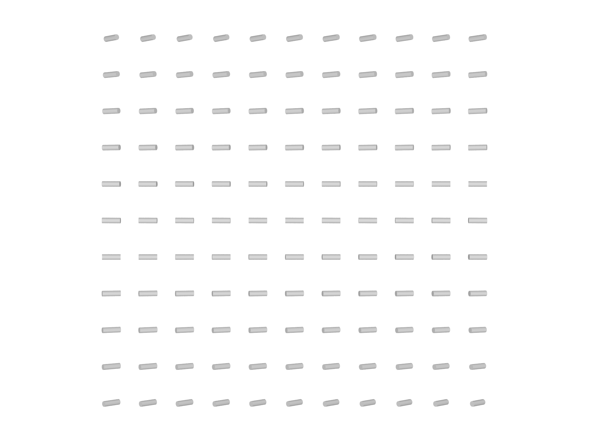
display a single director is as a cylinder oriented along \(\mathbf{n}\).
We will therefore make a helper function that creates a Graphics
object and draws such a cylinder at every mesh point:
// Function to visualize a director field
// m - the mesh
// nn - the director Field to visualize
// dl - scale the director
fn visualize(m, nn, dl) {
    var v = m.vertexmatrix()
    var nv = m.count() // Number of vertices
    var g = Graphics() // Create a graphics object
    for (i in 0...nv) {
    var x = v.column(i) // Get the ith vertex
    // Draw a cylinder aligned with nn at this vertex
    g.display(Cylinder(x-nn[i]*dl, x+nn[i]*dl, aspectratio=0.3))
    }
    return g
}
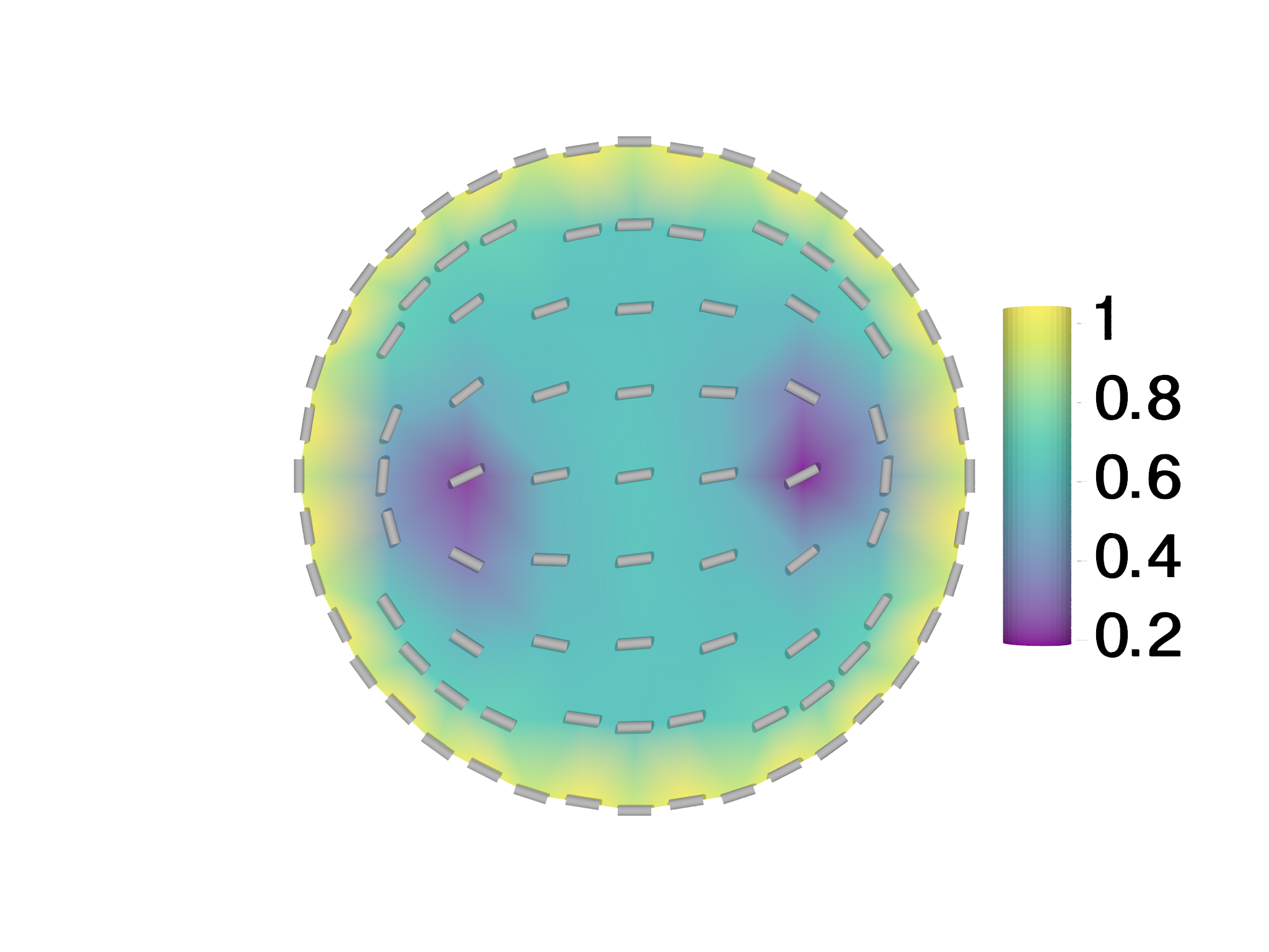
Once we've defined this function, we can use it:
var gnn=visualize(m, nn, 0.2)
The variables \(g\) and \(gnn\) now refer to two separate Graphics objects. We can combine them using the \(+\) operator, and display them like so:
var gdisp = g+gnn
Show(gdisp)

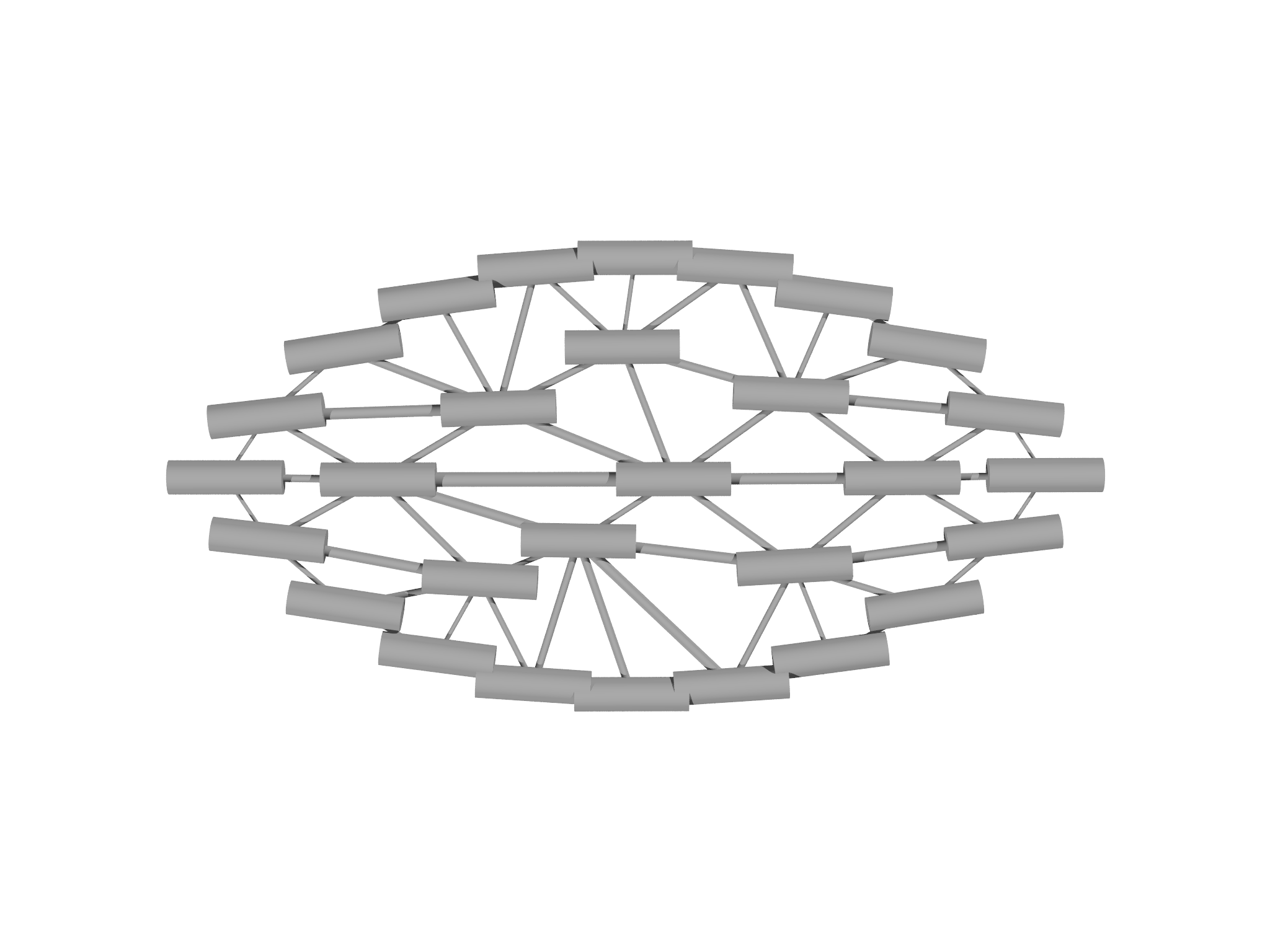
The resulting visualization is shown in Fig. 4.5.
Refinement
We have now solved our first shape optimization problem, and the
complete problem script is provided in the examples/tutorial folder
inside the git repository as tutorial.morpho. The result we have
obtained in Fig. 4.5 is, however, a very coarse, low resolution
solution comprising only a relatively small number of elements. To gain
an improved solution, we need to refine our mesh. Because modifying
the mesh also requires us to update other data structures like fields
and selections, a special MeshRefiner object is used to perform the
refinement.
To perform refinement we:
- Create a
MeshRefinerobject, providing it a list of all theMesh,FieldandSelectionobjects (i.e. the mesh and objects that directly depend on it) that need to be updated:var mr = MeshRefiner([m, nn, bnd]); // Set the refiner up - Call the
refinemethod on theMeshRefinerobject to actually perform the refinement. This method returns aDictionaryobject that maps the old objects to potentially newly created ones.var refmap = mr.refine(); // Perform the refinement - Tell any other objects that refer to the mesh, fields or selections
to update their references using
refmap. For example,OptimizationProblemandOptimizerobjects are typically updated at this step.for (el in [problem, sopt, fopt]) el.update(refmap); // Update the problem - Update our own references
m = refmap[m];
nn = refmap[nn];
bnd = refmap[bnd]; // Update variables
We insert this code after our optimization section, which causes morpho to successively optimize and refine.
The complete code including refinement is in
examples/tutorialfolder inside the git repository astutorial2.morpho
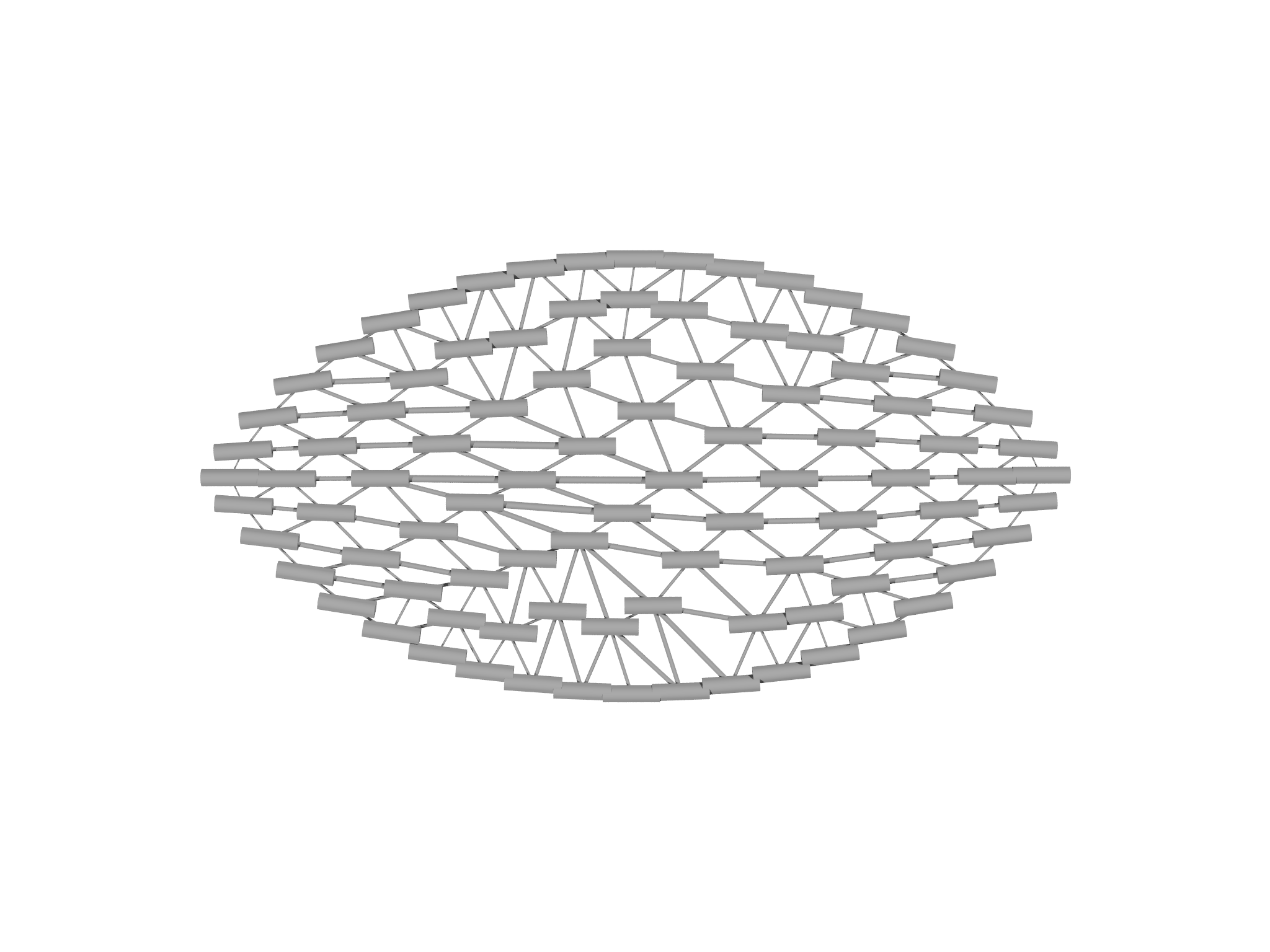
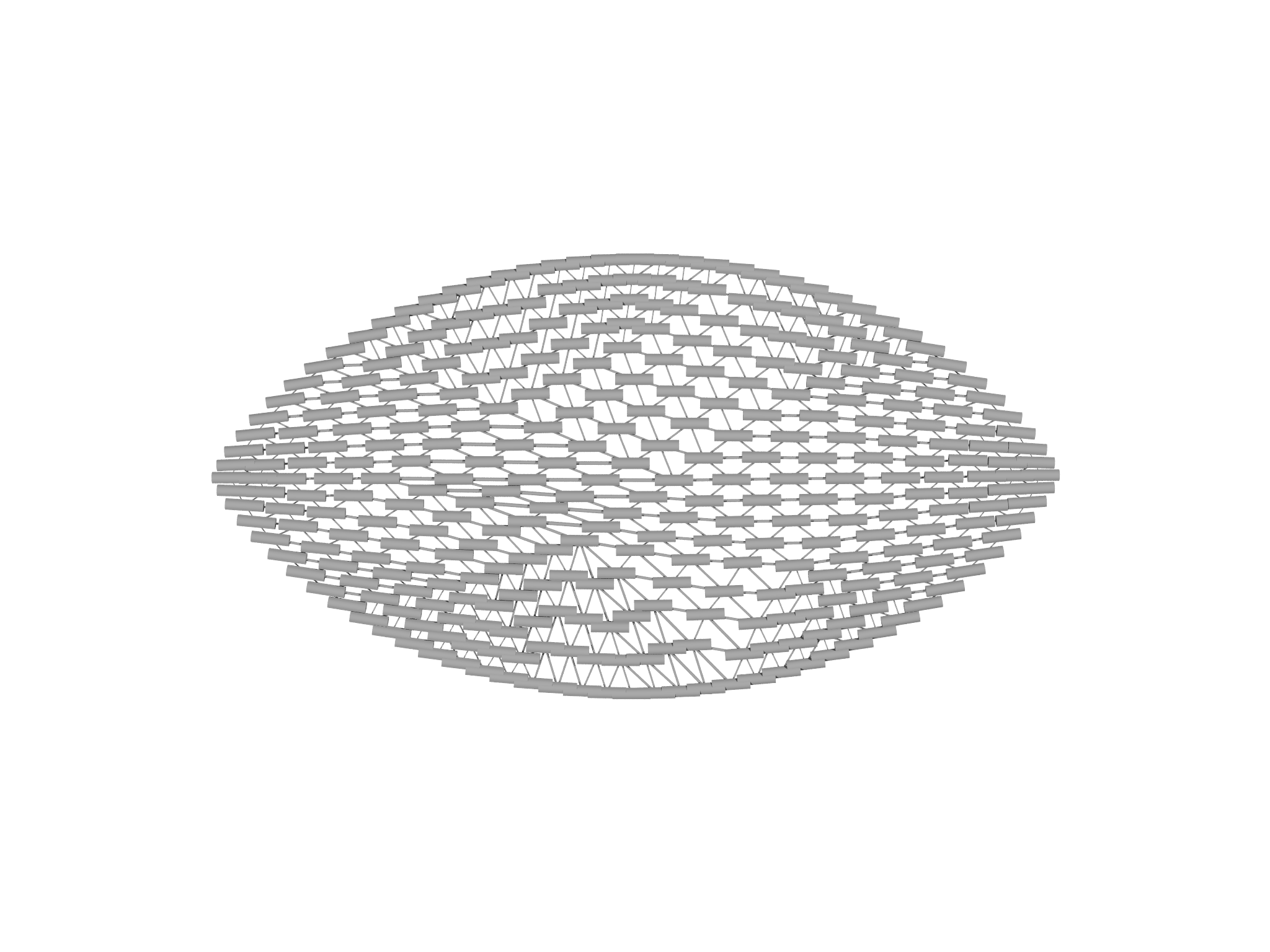
The resulting optimized shapes are displayed in Fig. 4.6.
// Optimization loop
var refmax = 3
for (refiter in 1..refmax) {
  print "===Refinement level ${refiter}==="
  for (i in 1..100) {
    fopt.linesearch(20)
    sopt.linesearch(20)
  }

  if (refiter==refmax) break

  // Refinement
  var mr=MeshRefiner([m, nn, bnd]) // Set the refiner up
  var refmap=mr.refine() // Perform the refinement
  for (el in [problem, sopt, fopt]) el.update(refmap) // Update the problem
  m=refmap[m]; nn=refmap[nn]; bnd=refmap[bnd] // Update variables
}
Next steps
Having completed this tutorial, you may wish to explore the effect of
changing some of the parameters in the file. What happens if you change
sigma and W, the coefficients in front of the terms in the energy?
What happens if you take a different number of steps? Or change
properties of the Optimizers like stepsize and steplimit?
You should look at other example files provided in the examples folder
of the git repository. The remainder of the manual comprises chapters
exploring certain morpho concepts in more detail, followed by a
detailed reference manual for morpho functionality, and a complete
description of the scripting language.
Working with Meshes
This chapter explains a number of ways the user can create and
manipulate Mesh objects in morpho. The simplest way to create a mesh
for a desired domain is to use the meshgen module, which provides a
very high level and convenient interface. The meshtools module
provides low level mesh creation operations and a number of useful
routines to manipulate meshes. The implicitmesh module produces
surfaces from implicit functions. Finally, you can use an external
program to create a mesh that exports the data in vtk format using the
vtk module.
Mesh creation follows two patterns. Some methods use a constructor pattern where you call a single function that creates the Mesh, e.g.
var mesh = LineMesh(fn (t) [t,0], -1..1:0.1)
Other approaches follow a builder pattern, where you first create a special helper object,
var mb = MeshBuilder()
and manipulate it, e.g. by adding elements or setting options. The Mesh is then created by calling the build method:
var mesh = mb.build()
The meshgen module
The meshgen module conveniently produces high quality meshes for many
kinds of domain. It follows the builder pattern with a MeshGen helper
object that performs the construction. To use meshgen, the user must
provide a scalar function that is positive everywhere that they want to
be meshed.
Note One example is referred to in the literature as a signed distance function, which is the Euclidean distance of a given point \(x\) to the boundary of a set \(\Omega\) with the sign positive if \(x\) is in the interior of \(\Omega\). MeshGen does not require signed distance functions, but accepts any continuous and reasonably smooth function.
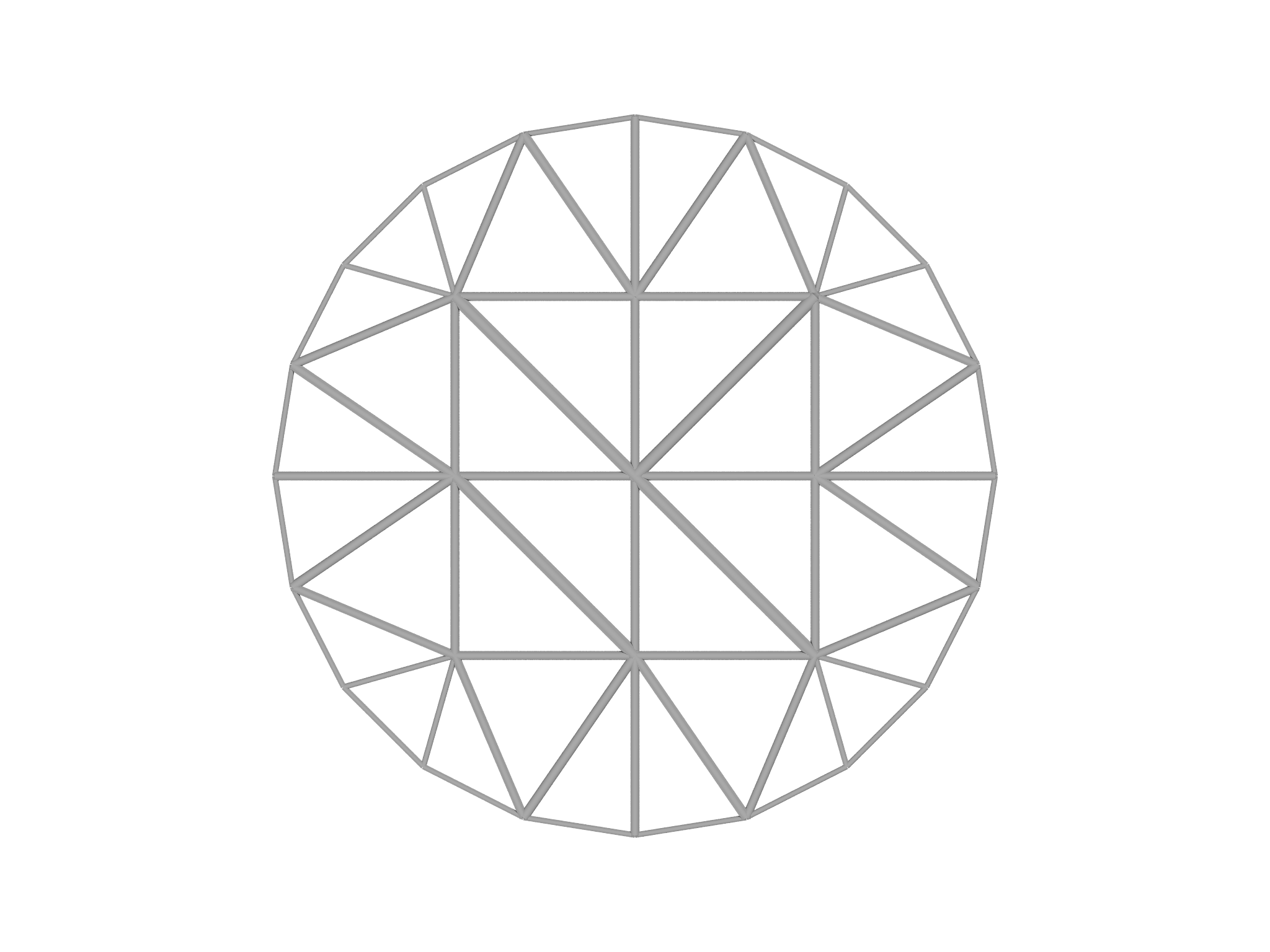
For example, the interior of the unit disk in two
dimensions, is described by the function $$f(x,y)=1-(x^{2}+y^{2}).$$ To
create the corresponding Mesh, we must first specify a suitable morpho
function that describes the domain. This function will be called
repeatedly by MeshGen, which will pass it a position vector x. Hence,
the \((x,y)\) components must be accessed from the argument x by
indexing:
fn disk(x) {
    return 1-(x[0]^2+x[1]^2)
}
Now that the function is specified, we can create a MeshGen object:
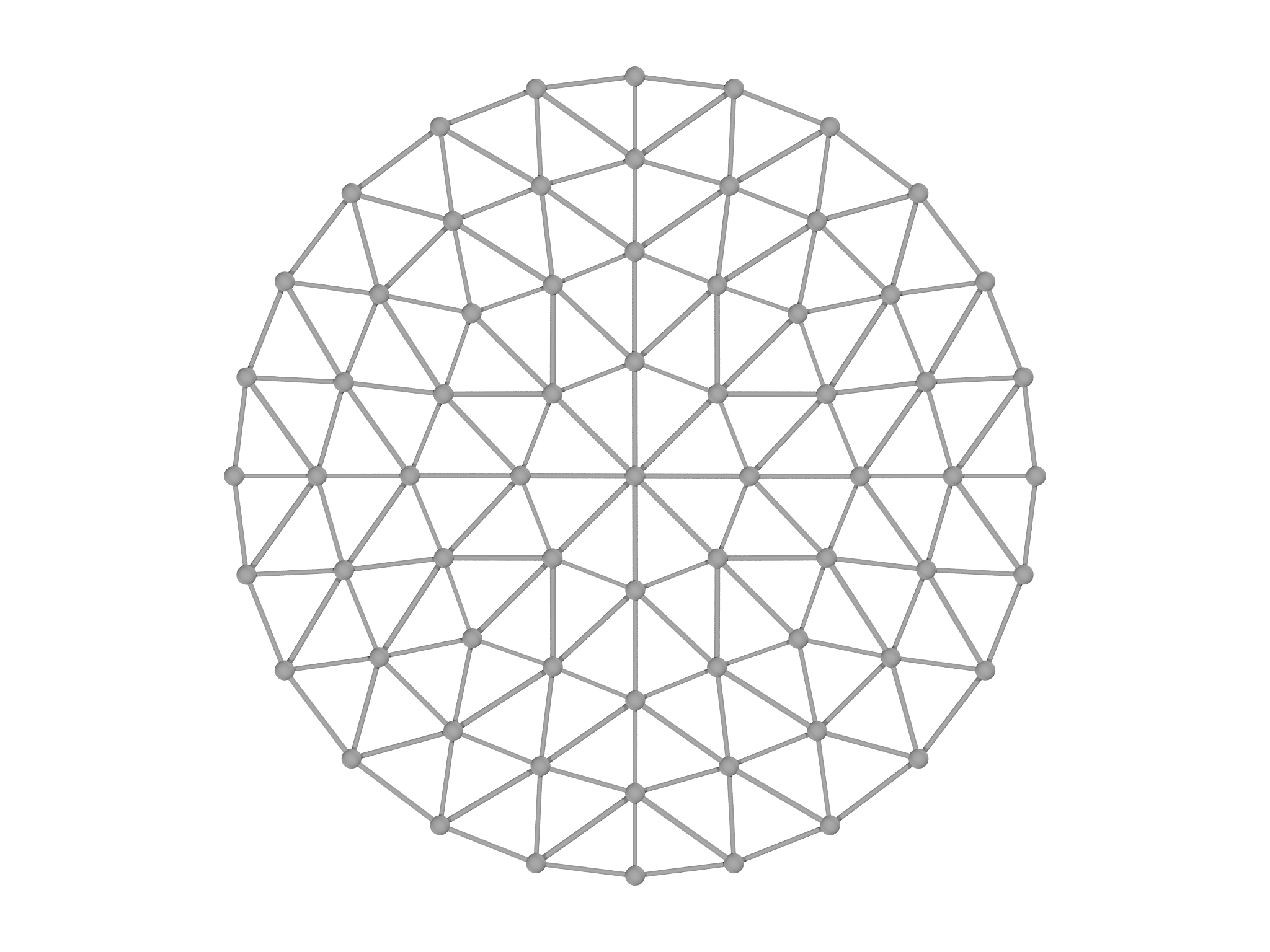
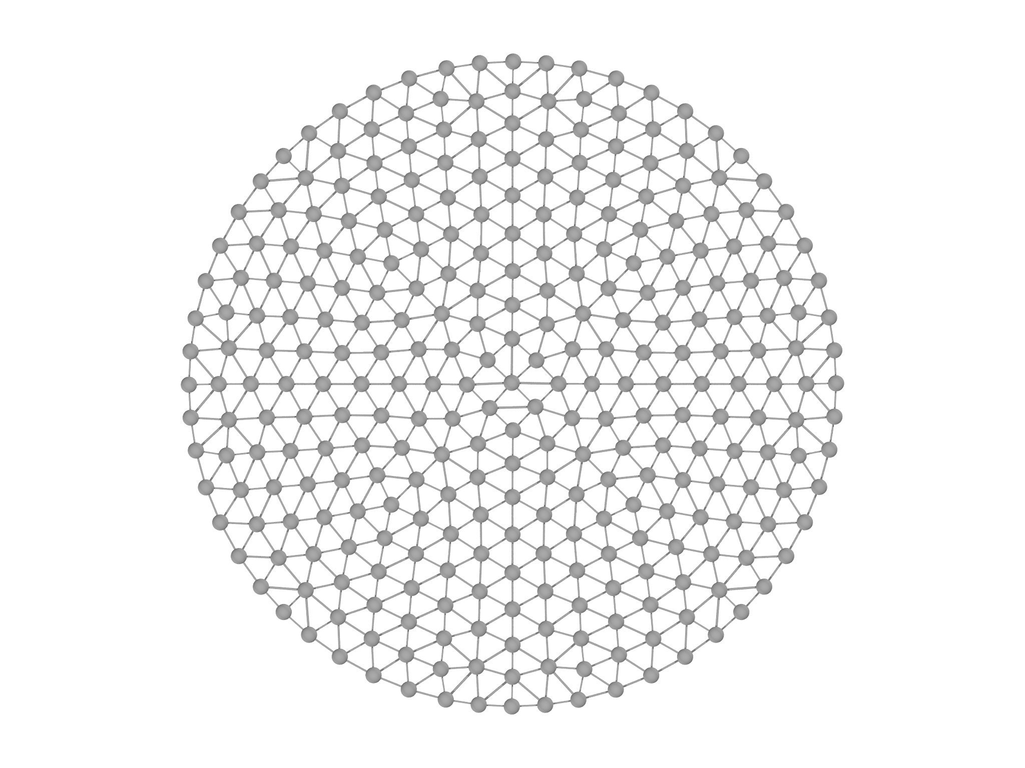
var mg = MeshGen(disk, [-1..1:0.2, -1..1:0.2])
The second parameter is a list of Ranges that provide overall bounds on the domain to be meshed. Here we will use \(x,y\in[-1,1]\). By setting the stepsize, the user can provide MeshGen with an overall suggestion of the resolution.
Finally, we create the Mesh by calling the build method:
var m = mg.build();
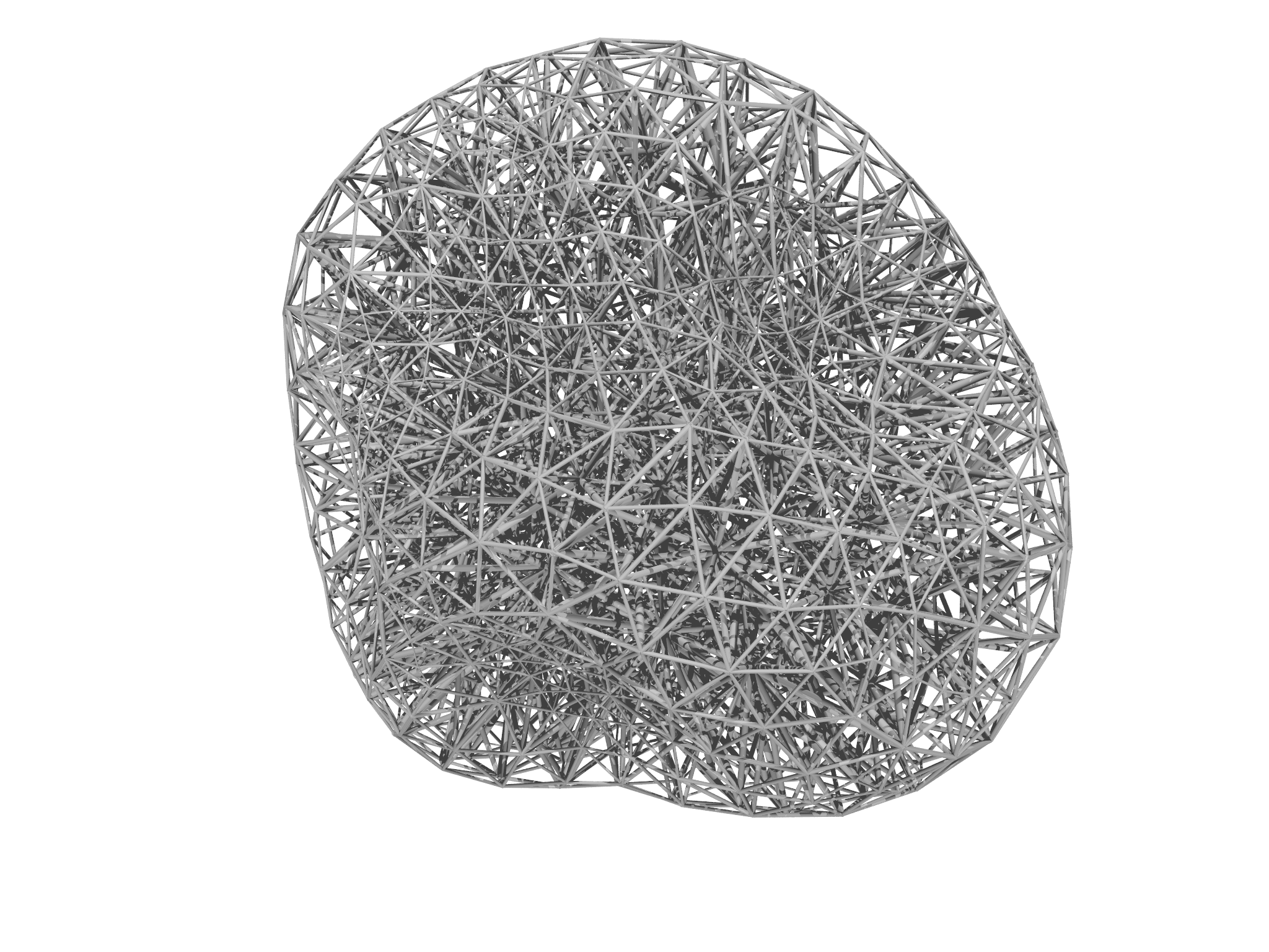
The resulting Mesh is shown in Fig. 5.1, left panel. A higher resolution Mesh can be generated by changing the Range objects passed to MeshGen:
var mg = MeshGen(disk, [-1..1:0.1, -1..1:0.1])
This generates a much higher resolution Mesh, with approximately four times the number of vertices as shown in Fig. 5.1, right panel.
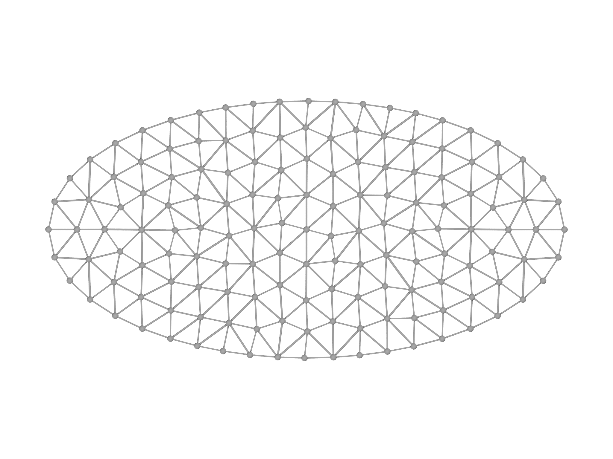
MeshGen can also mesh more complicated domains. To facilitate this, it provides a Domain class that accepts a scalar function in its constructor. For example, this code creates an ellipse as shown in Fig. 5.2, left panel:
var e0 = Domain(fn (x) -((x[0]/2)^2+x[1]^2-1))
var mg = MeshGen(e0, [-2..2:0.2, -1..1:0.2])
var m = mg.build()
The benefit of this is that Domain objects can be combined using set
operation methods union, intersection and difference. To
illustrate the possibilities with this, we use a special constructor to
create three domains corresponding to disks,
var a = CircularDomain(Matrix([-0.5,0]), 1)
var b = CircularDomain(Matrix([0.5,0]), 1)
var c = CircularDomain(Matrix([0,0]), 0.3)
then combine them,
var dom = a.union(b).difference(c)
and mesh the resulting domain,
var mg = MeshGen(dom, [-2..2:0.1, -1..1:0.1], quiet=false)
var m = mg.build()
with the result shown in Fig. 5.2, right panel.

Three dimensional meshes are created very similarly. Here we create a spherical mesh, displayed in Fig. 5.3
var dh = 0.2
var dom = Domain(fn (x) -(x[0]^2+x[1]^2+x[2]^2-1))
var mg = MeshGen(dom, [-1..1:dh, -1..1:dh, -1..1:dh])
var m = mg.build()
The meshtools module
Meshtools provides many useful functions for working with Meshes, including constructors to create certain kinds of Mesh and also classes for refining, coarsening and merging Meshes.
LineMesh
The LineMesh function is a convenient way to create a Mesh from a
one-parameter parametric function. You must specify the function to use
and a Range of points to generate. LineMesh then evaluates each point
in the Range and joins them together with a line element.
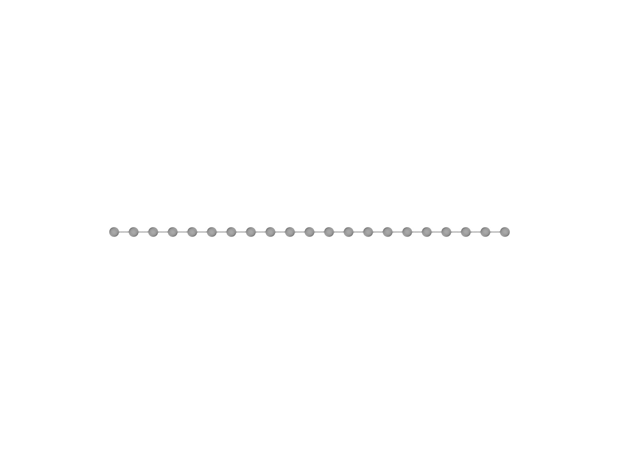
This is useful to generate meshes such as a simple straight line (Fig. 5.4, left panel):
var m = LineMesh(fn (t) [t,0], -1..1:0.1)
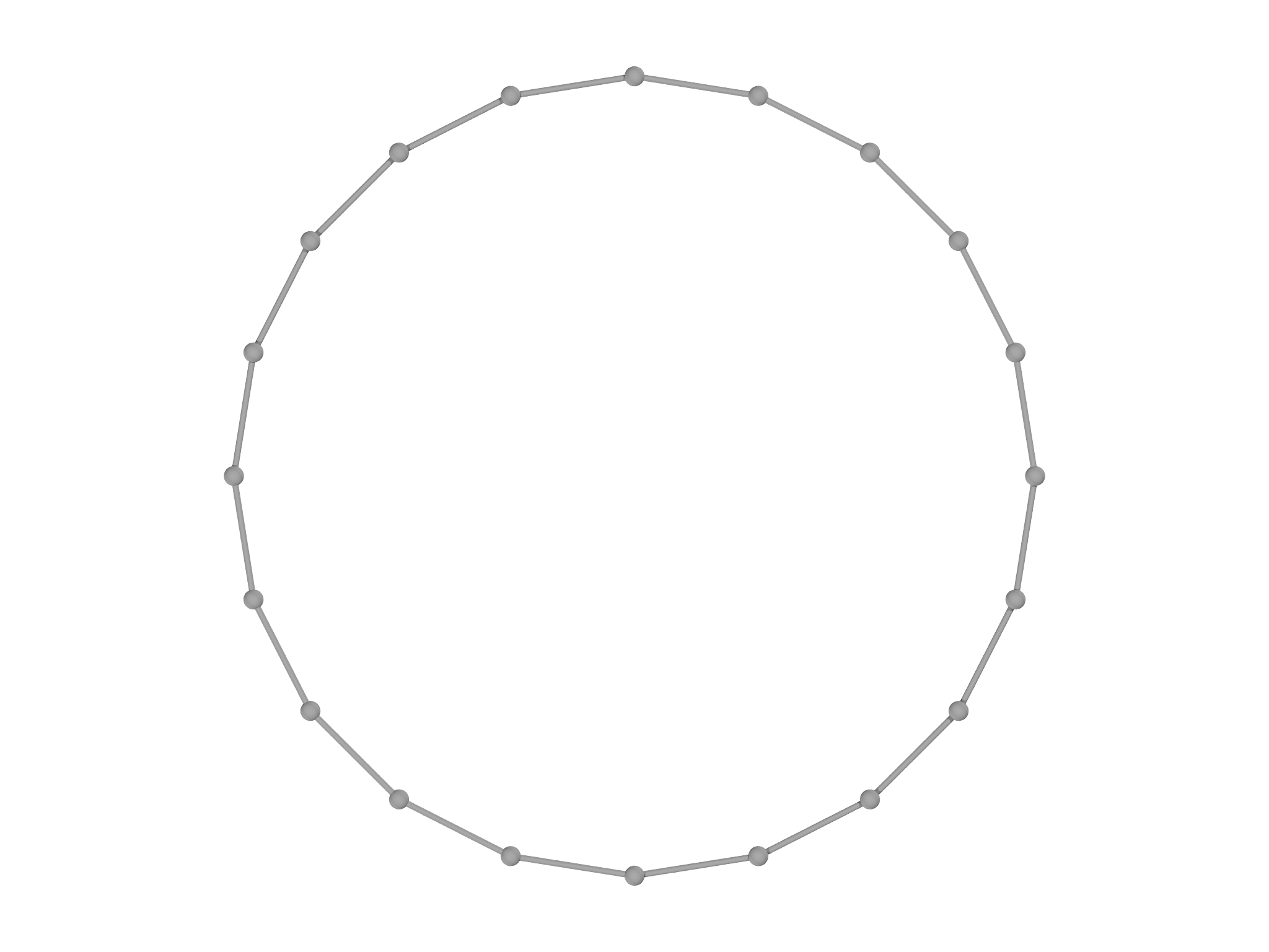
You can also request the ends of the Mesh be joined together to form a
loop by specifying closed. This code generates a circle (Fig.
5.4,
center panel):
var m = LineMesh(fn (t) [cos(t),sin(t)], -Pi...Pi:2*Pi/10, closed=true)
You can increase the resolution of the circle by changing the stepsize
in the Range, for example to 2``*``Pi/20 to double the number of
points. Note the use of the exclusive Range operator here, ..., rather
than ..to avoid duplicating the point at (1,0).
The output Mesh can be of any dimension, such as this helix in 3D (Fig. 5.4, right panel). Notice that here we use a regular function rather than an anonymous function:
fn helix(t) {
  return [cos(2*Pi*t),t/2,sin(2*Pi*t)]
}
var m = LineMesh(helix, -2..2:1/20)

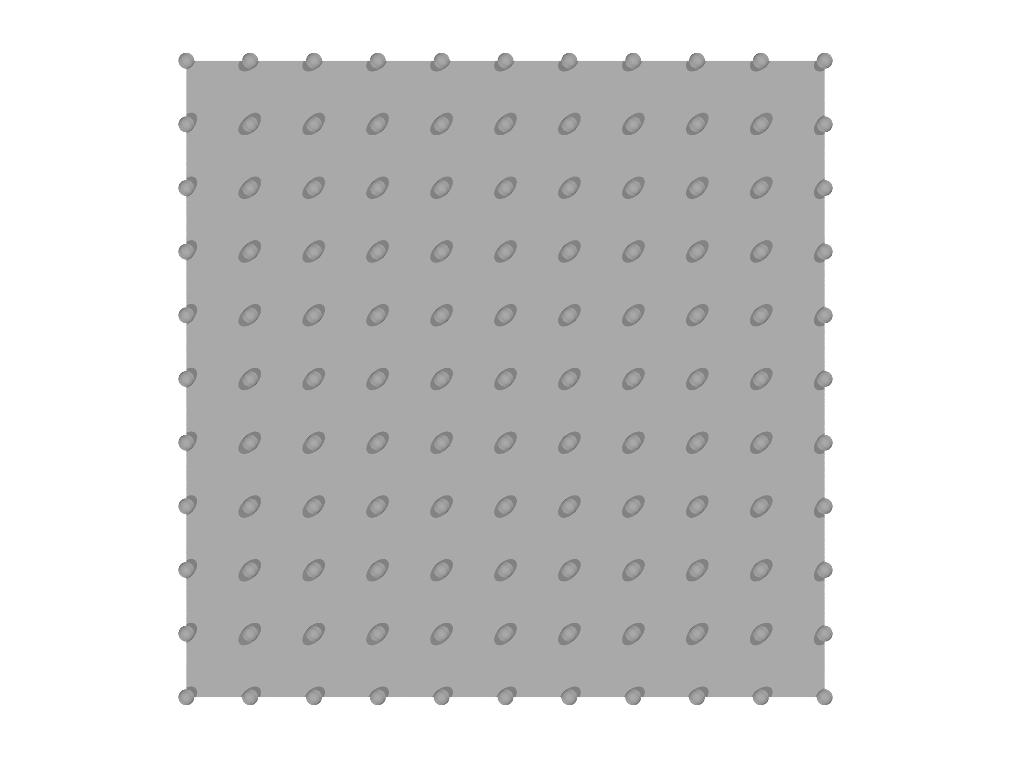
AreaMesh
AreaMesh is similar to LineMesh function creates a Mesh from a
parametric function, which now takes two parameters. To create a square,
var m = AreaMesh(fn (u,v) [u,v,0], -1..1:0.2, -1..1:0.2)
where notice that a separate Range is required for \(u\) and \(v\). By
default, the output of AreaMesh only contains grade 0 and grade 2
elements, i.e. vertices and facets, as is visible in Fig.
5.5(left). To add in grade 1 elements if
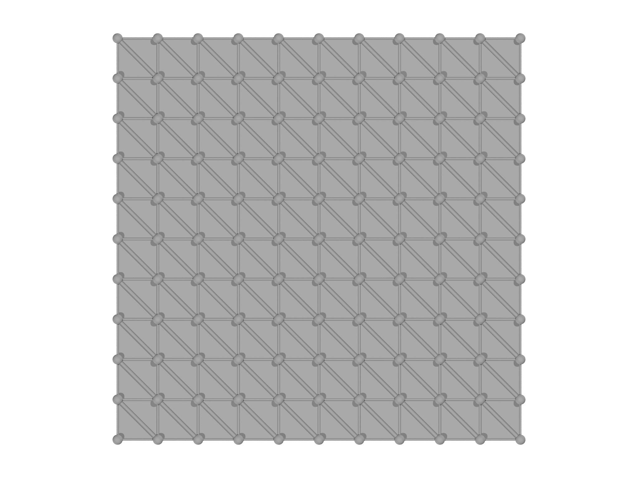
required, call the addgrade method on the Mesh:
m.addgrade(1)
This gives the result shown in Fig. [5.5](#fig:AreaMesh-1(right).
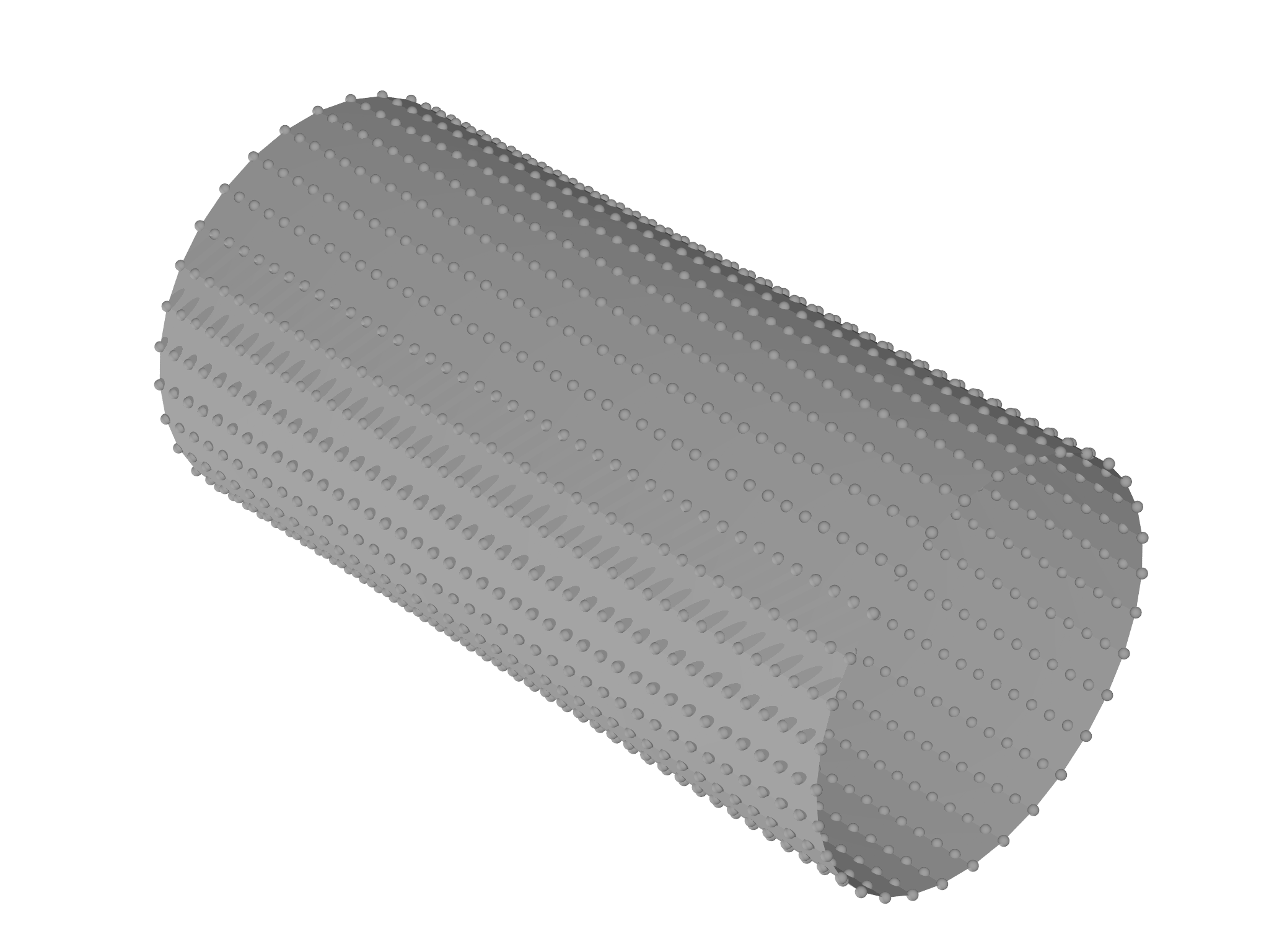
addgrade.As with LineMesh, the Meshes can be closed in one or both directions, enabling the creation of a cylinder,
m = AreaMesh(fn (u, v) [v, cos(u), sin(u)],
               -Pi...Pi:Pi/16,
               -2..2:0.1, closed=[true, false])
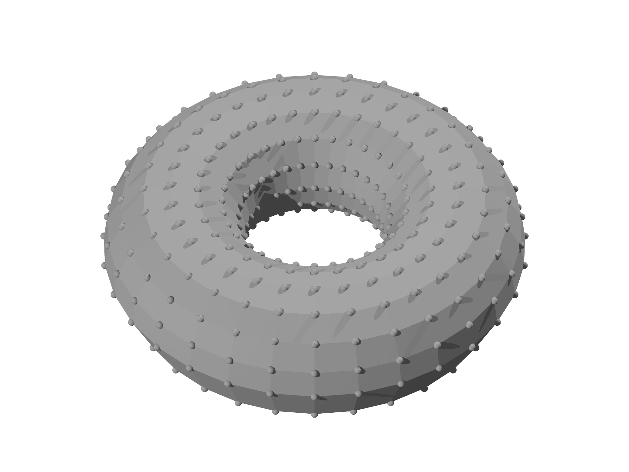
and a torus,
var c=1, a=0.5 m = AreaMesh(fn (u, v) [(c + a*cos(v))*cos(u),
                                       (c + a*cos(v))*sin(u),
                                        a*sin(v)],
                            0...2*Pi:Pi/16,
                            0...2*Pi:Pi/8, closed=true)
The results of these are displayed in Fig.
5.6.
Note that the meshes generated by more modules that incorporate some
degree of quality control, e.g. implicitmesh or meshgen, are
generally better and should be used in preference to those created by
AreaMesh.
PolyhedronMesh
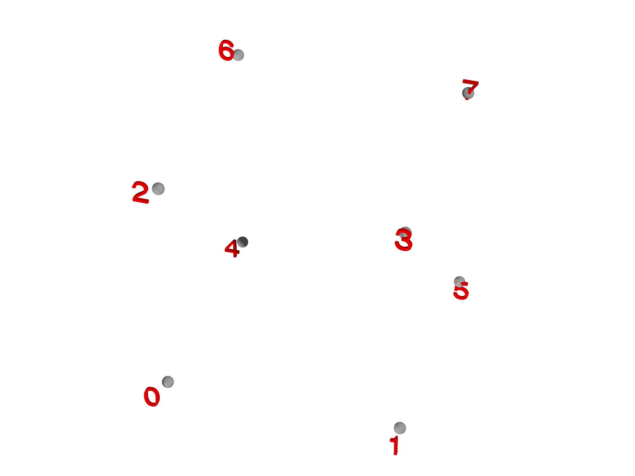

PolyhedronMesh helps to create Meshes corresponding to polyhedra. To make a cube, for example, we specify the eight vertices (see Fig. 5.7, left),
var vertices = [[-0.5, -0.5, -0.5],
                [ 0.5, -0.5, -0.5],
                [-0.5,  0.5, -0.5],
                [ 0.5,  0.5, -0.5],
                [-0.5, -0.5,  0.5],
                [ 0.5, -0.5,  0.5],
                [-0.5,  0.5,  0.5],
                [ 0.5,  0.5,  0.5]]
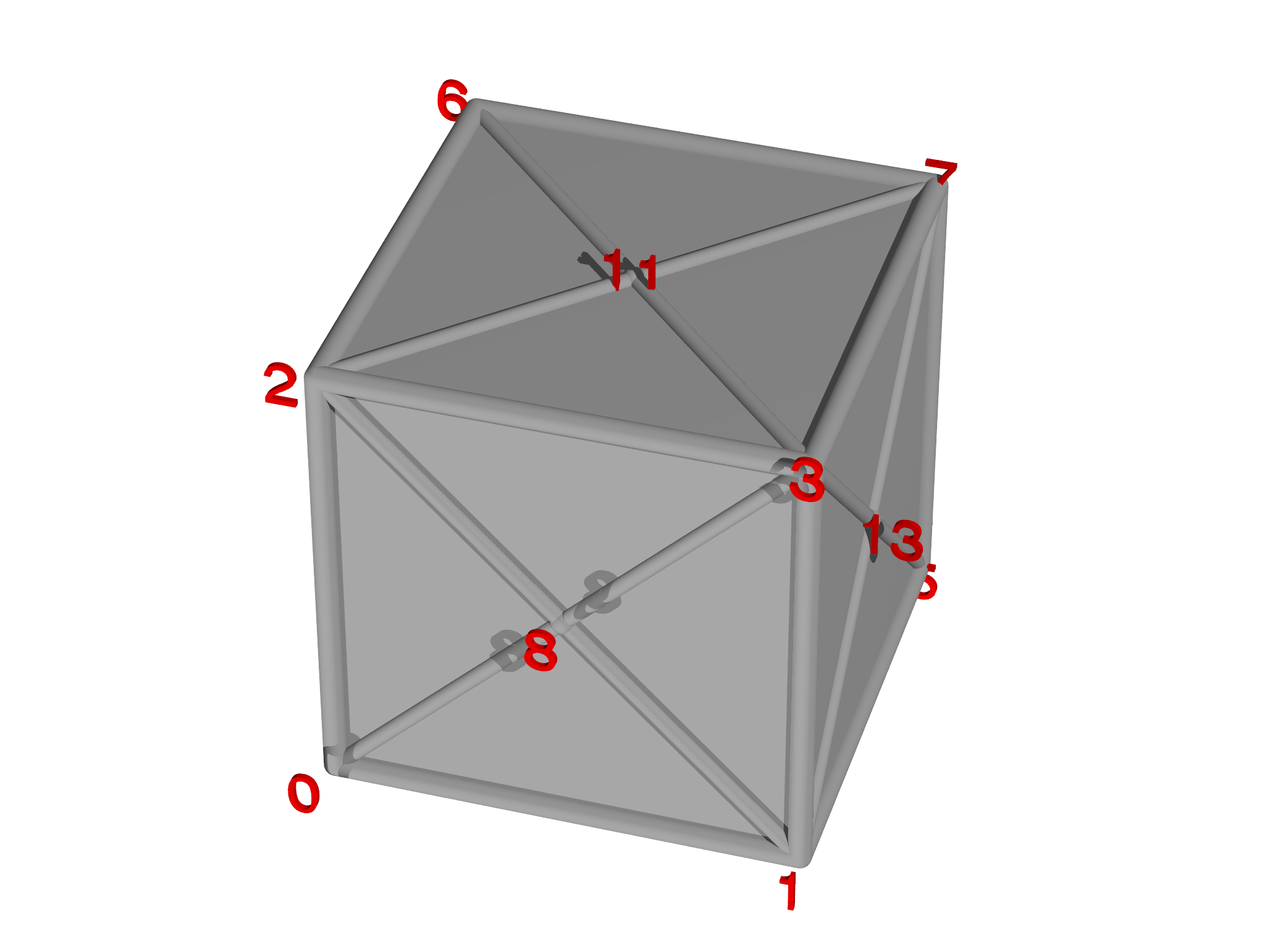
and the six faces,
var faces = [ [0,1,3,2], [4,5,7,6],
              [0,1,5,4], [3,2,6,7],
              [0,2,6,4], [1,3,7,5] ]
Note that the vertex ids must be given in order going around each face (see Fig. 5.7{reference-type="ref" reference="fig:PolyhedronMesh"}, center). Once the faces are specified, we can create the mesh,
var m = PolyhedronMesh(vertices, faces)
m.addgrade(1)
Note that PolyhedronMesh automatically creates additional vertices and generates triangles to complete the mesh (Fig. 5.7, right). We then added line elements (grade 1) as these are not automatically created by PolyhedronMesh.
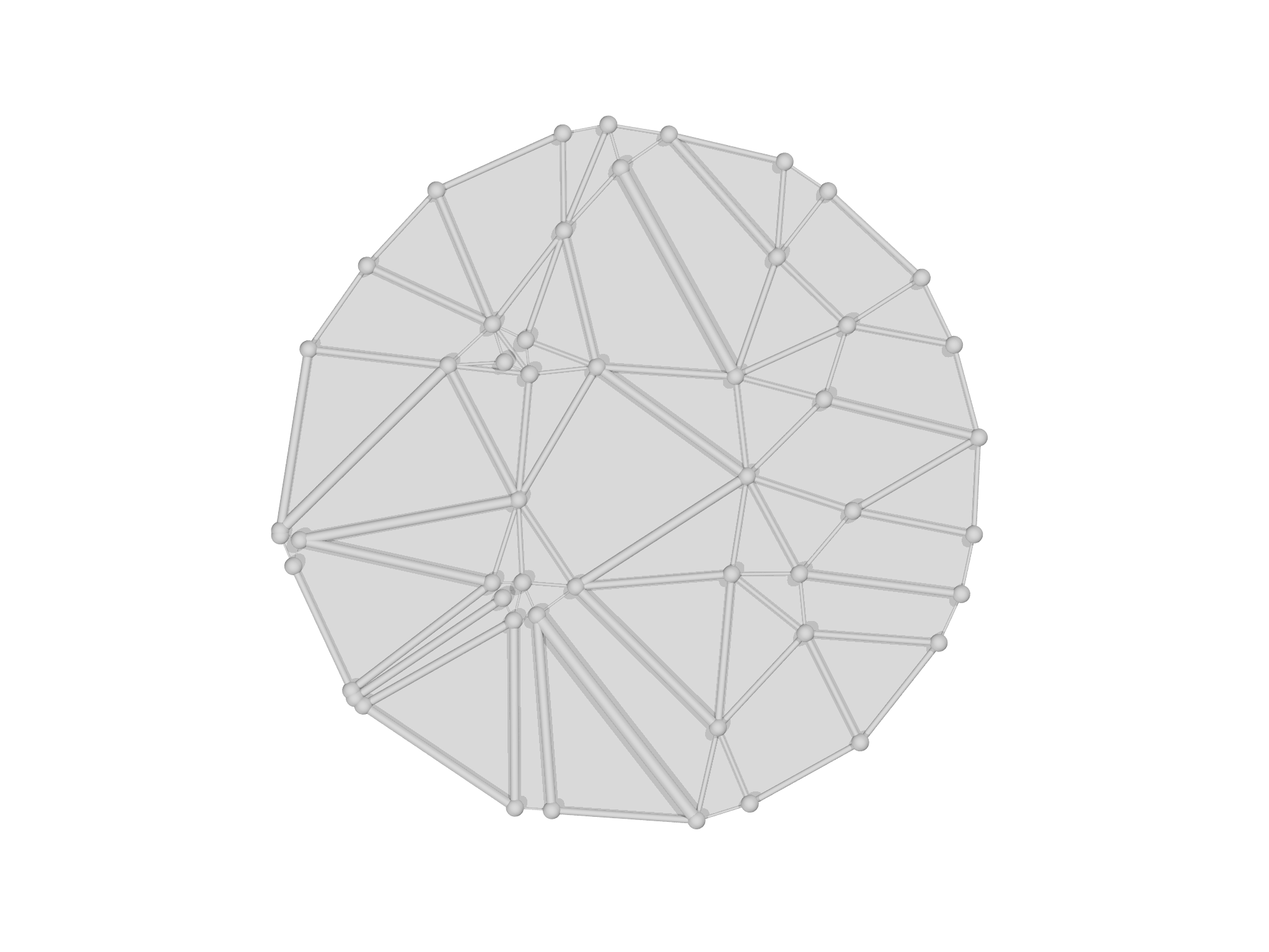
DelaunayMesh

The DelaunayMesh constructor function performs a delaunay "triangulation" of a point set. For example, creating a random cloud of points (Fig. 5.8, left panel):
var pts = []
for (i in 0...100) pts.append(Matrix([2*random()-1, 2*random()-1, 2*random()-1]))
we can then call DelaunayMesh to construct a tetrahedralization.
DelaunayMesh only generates elements of the highest grade (in 2D, area
elements, in 3D volume elements) so if edges are needed these can be
added with addgrade.
var m=DelaunayMesh(pts)
m.addgrade(1)
The resulting tetrahedralization is shown in Fig. 5.8, right panel.
ChangeMeshDimension
Occasionally, one wishes to take a mesh embedded in one space, say two
dimensions, and embed it in a space of different dimensionality. For
example, you may wish to use a 2D mesh generated with MeshGen in 3D
space. The function ChangeMeshDimension provides a convenient way to
do this:
var new = ChangeMeshDimension(mesh, dim)
where dim is the target dimension of the new mesh.
MeshBuilder
The MeshBuilder class facilitates manual construction of a Mesh object. It is primarily intended to be used by other mesh building algorithms, but is occasionally useful. To begin, create a MeshBuilder object:
var mb = MeshBuilder()
You can then add vertices and other elements one by one by calling appropriate methods. Let's build a tetrahedron by first adding the vertices:
mb.addvertex([0, 0, 0.612372])
mb.addvertex([-0.288675, -0.5, -0.204124])
mb.addvertex([-0.288675, 0.5, -0.204124])
mb.addvertex([0.57735, 0, -0.204124])
We then need to add edges connecting these vertices, and faces as well. We could do this one by one, giving a list of vertex ids for each element in turn,
mb.addedge([0,1])
mb.addedge([0,2])
// ... etc.
but there's a smarter way for this case. Notice that the vertex ids
corresponding to the edges of the tetrahedron correspond to the sets of
size 2 generated from the list [``0,1,2,3``] as can be seen by running
this code:
var vids = [0,1,2,3]
for (s in vids.sets(2)) print s
We can therefore generate the edges automatically,
var vids = [0,1,2,3]
for (s in vids.sets(2)) mb.addedge(s)
and the faces as well, which are the sets of size 3,
for (s in vids.sets(3)) mb.addface(s)
We can finish by adding a single grade 3 element corresponding to the volume:
mb.addvolume(vids)
Once all these have been added, call the build method to create a Mesh
object:
var m = mb.build()
and the resulting Mesh is shown in Fig. 5.9.

The vtk module
The vtk module provides importing and exporting facilities for the
popular VTK file format, which is used by many other programs such as
paraview. Unlike morpho .mesh files, VTK files can include both Mesh
and Field data. To load a mesh from a VTK file, use a VTKImporter
object:
import vtk
var mv = VTKImporter("file.vtk")
var m = mv.mesh()
Fields can be loaded in a similar way. Each field in the VTK file has an
identifier, which is passed to the field method as a string.
var f = mv.field("F")
var g = mv.field("G")
Exporting requires a VTKExporter class,
import meshtools
import vtk
var m1 = LineMesh(fn (t) [t,0,0], -1..1:2)
var g1 = Field(m1, fn(x,y,z) Matrix([x,2*x,3*x]))

var vtkE = VTKExporter(g1, fieldname="g")
vtkE.export("data.vtk")
Merging meshes
A potential strategy to create meshes for complicated domains is to
begin by creating several simpler meshes and then merging them together
into one larger mesh. The MeshMerge class in the meshtools package
allows us to do this. To use it, we create a MeshMerge object with a
list of meshes we wish to merge
var mrg = MeshMerge([m1, m2, m3, ... ])
and then call the merge method to perform the merge and return the resulting Mesh:
var newmesh = mrg.merge()
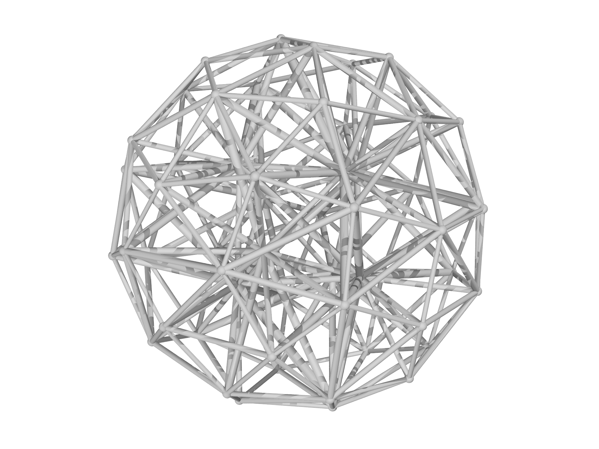
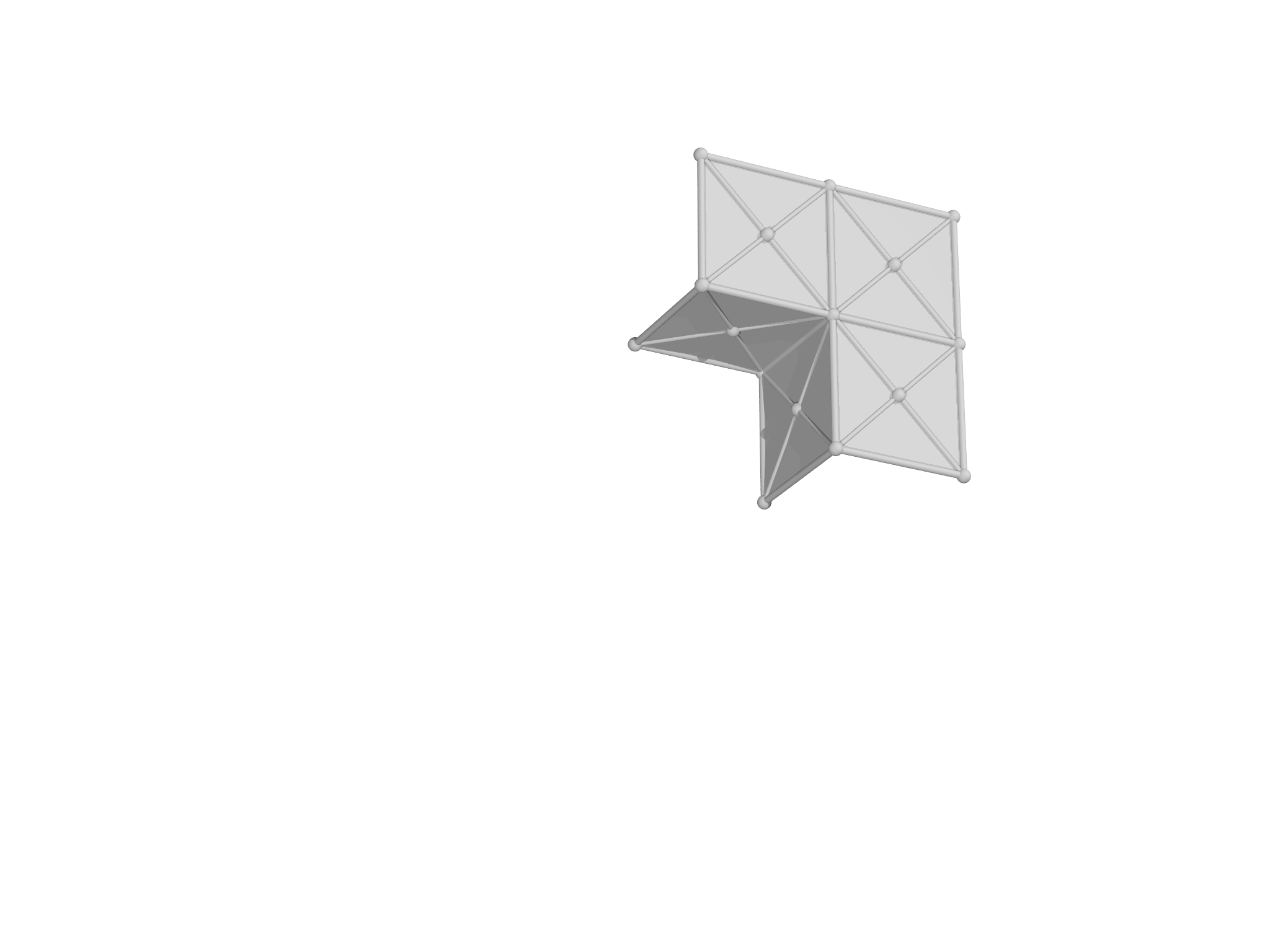
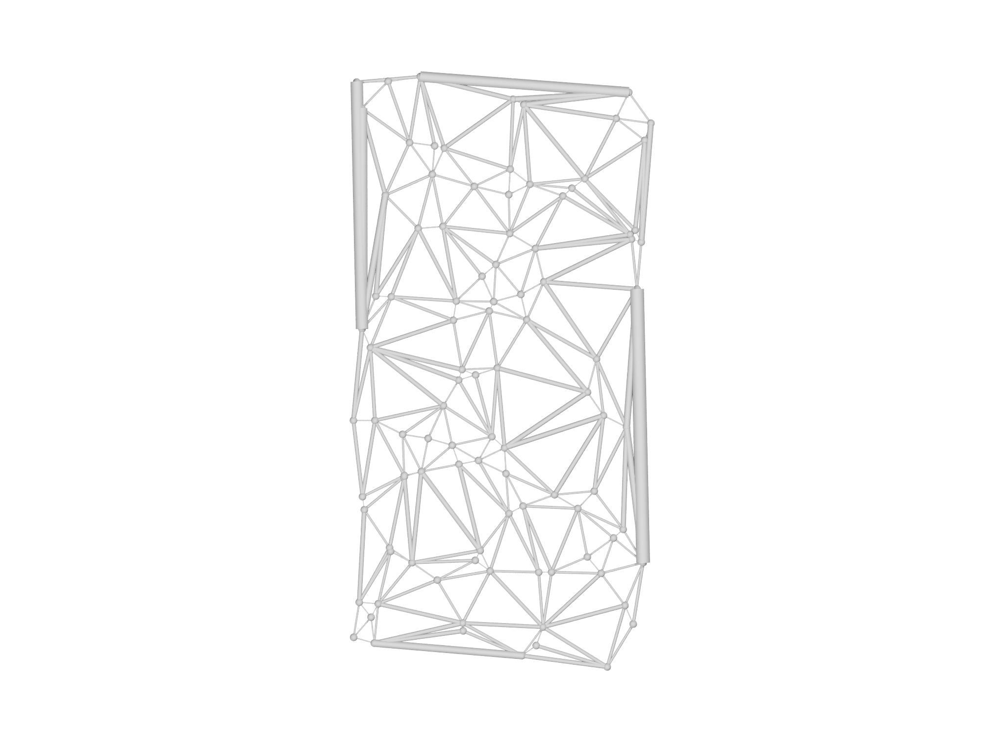
As an example of this, we will build a mesh that might be an initial guess for a membrane held between two square fixed boundaries. We'll do this by creating one octant and then reflecting it along different axes. The basic unit is constructed with PolyhedronMesh, as shown in Fig. 5.11:
var a = 0.5 // Vertical separation
var r = 0.5 // Size of hole
var L = 1  // Size of box

// One octant of the mesh
var vertices = [ [r,0,a], [L,0,a], [L,r,a], [L,L,a],
                 [r,L,a], [0,L,a], [0,r,a], [r,r,a],
                 [r,0,0], [r,r,0], [0,r,0] ]
var faces = [ [0,1,2,7], [2,3,4,7], [7,4,5,6], [0,8,9,7], [6,7,9,10] ]

var m1 = PolyhedronMesh(vertices, faces)
m1.addgrade(1)
We now need to create code that reflects a Mesh about one or more axes. There's more than one way this could be done, but we will here create a MeshReflector class that follows the builder pattern:
class MeshReflector {
  init(mesh) {
    self.mesh = mesh
    self.dim = mesh.vertexmatrix().dimensions()[0] // Get Mesh dimension
  }

  // Construct a matrix that reflects about one or more axes
  _reflectionmatrix(axis) {
    var rmat = Matrix(self.dim,self.dim)
    for (i in 0...self.dim) rmat[i,i]=1
    if (isint(axis)) rmat[axis,axis]*=-1
    else if (isobject(axis)) for (i in axis) rmat[i,i]*=-1
    return rmat
  }

  reflect(axis) { // Reflect the mesh about the given axis or axes
    var rmat = self._reflectionmatrix(axis)
    // Clone and transform the mesh
    var m = self.mesh.clone()
    for (vid in 0...m.count()) {
      m.setvertexposition(vid, rmat * m.vertexposition(vid))
    }
    return m
  }
}
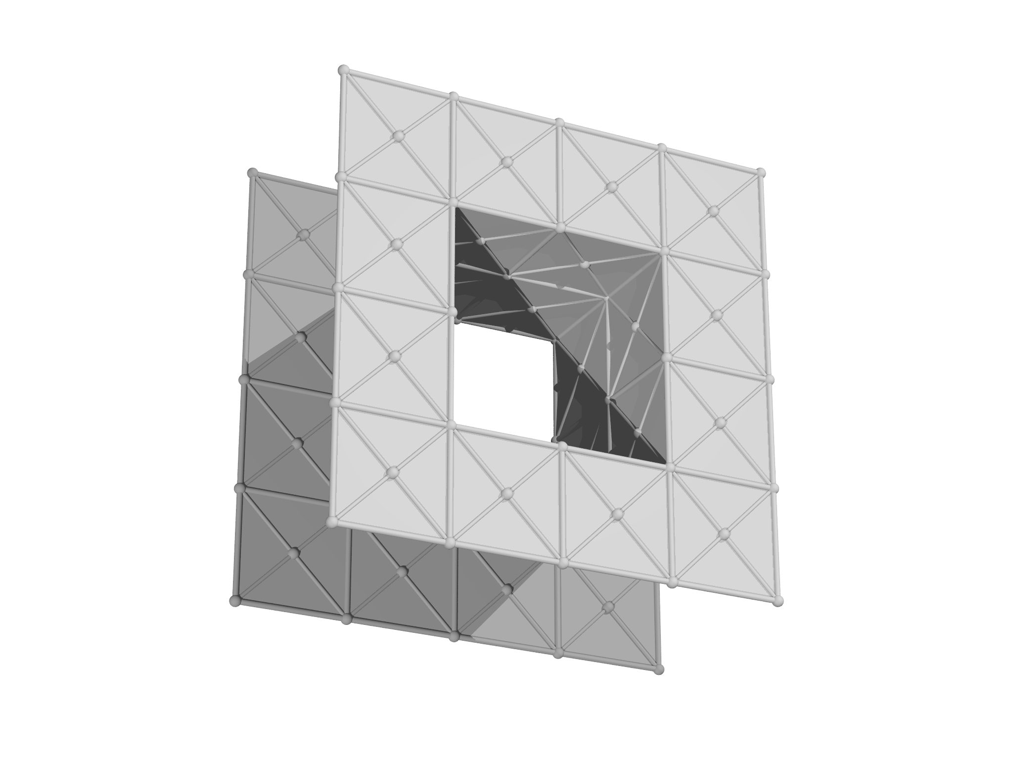
Having defined this class, we create a MeshReflector and use it to build seven reflected copies:
var mr = MeshReflector(m1)

// Merge reflected meshed together
var merge = MeshMerge([ m1,
                        mr.reflect(0),
                        mr.reflect(1),
                        mr.reflect(2),
                        mr.reflect([0,1]),
                        mr.reflect([1,2]),
                        mr.reflect([2,0]),
                        mr.reflect([0,1,2])
                      ])
var m = merge.merge()
The resulting mesh is shown in Fig. 5.11, right panel. Note that MeshMerge automatically removes duplicate elements as the merge is performed, so that
print m1.count(1)
reports that there were 35 line elements in the original mesh, while
print m.count(1)
yields \(256=8\times(35-6/2)\) line elements, because there are 6 shared edges for each copy.
Slicing meshes
The meshslice module is designed to help visualize a "slice" through
the mesh and associated Fields, which is often useful when working with
three or higher dimensional meshes. To illustrate its use, we'll reuse
the spherical mesh created with MeshGen in the Meshgen Section above (see Fig.
5.3).
Ensure that the mesh has grade 2 elements present with addgrade if
necessary. We'll also create a simple scalar field:
var u = Field(m, fn (x,y,z) x*y)
To take a slice, first create a MeshSlicer object with the mesh we want to slice:
var ms=MeshSlicer(m)
Then call the slice method, which requires us to specify a slicing
plane. Planes are defined by a point \((x,y,z)\) and a normal vector
\((n_{x},n_{y},n_{z})\), which are passed as arguments:
var slc=ms.slice([0,0,0],[0,0,1]) // position, normal
After taking a slice, we can then slice any number of Field objects as well:
var uslc=ms.slicefield(u)
A single MeshSlicer can take any number of slices from the same Mesh;
slicefield always uses the most recent slice taken. Results from the
example are shown in Fig. 5.12. As can be seen, the results of slicing a
Mesh typically produce meshes that are quire irregular, with narrow
triangles and unequally sized elements. Hence, these meshes are intended
mostly for visualization purposes rather than use in calculations.

Visualization
This chapter describes ways to use morpho to visualize output. Easy to
use functions to visualize geometric objects are found in the plot
module, while you can draw arbitrary objects using the graphics
module. Publication quality output can be generated conveniently using
the povray module.
The plot module
A B
B C
C
grade option. C The color of the mesh can
be chosen with the color option.The plot module offers a convenient way to visualize Meshes, Fields
and Selections. To illustrate its use, we'll create a simple Mesh,
import meshtools
var m = AreaMesh(fn (u,v) [u, v, 0], -1..1:0.2, -1..1:0.2)
m.addgrade(1)
and an associated scalar Field,
var f = Field(m, fn (x,y) x*y)
Meshes
To visualize the Mesh, use the plotmesh function
var g = plotmesh(m)
which outputs a Graphics object, which we'll describe more fully in
the Graphics Section below. By default, plotmesh shows
only the highest grade element presenthere grade 2 or facetsas shown in
Fig. 6.1A. To show other grades, use the grade
option:
var g = plotmesh(m, grade=[0,1])
which shows points and edges as shown in Fig. 6.1B.
You can control the color of the Mesh with the color option as shown
in Fig. 6.1C:
var g = plotmesh(m, grade=0, color=Red)
To display particular selected elements of a mesh, you can use the
optional selection argument and supply a Selection object.
var sel = Selection(m, fn (x,y,z) x^2+y^2<1)
sel.addgrade(2)
var g = plotmesh(m, grade=[0,2], selection=sel)
Mesh labels
A B
B
It's sometimes helpful to be able to identify the id of a particular
element in a Mesh, especially for debugging purposes. The
plotmeshlabels function is designed to facilitate this as shown in
Fig. 6.2. You can select which grade to draw ids
for and specify their color, size and draw direction. It's also possible
to give an offset, which can be a list, matrix or even a function, that
adjusts the placement of the labels relative to the center of the
element. Here we offset them a little above and to the right:
var glabel = plotmeshlabels(m, grade=0, color=Black, offset=[0.025,0.025,0])
The plotmeshlabels function only draws labels, not the mesh itself, so
we typically combine it with plotmesh and display both:
var gmesh = plotmesh(m, grade=[0,1])
var g = gmesh+glabel
To show the grade 1 element ids, for example, we might use:
var glabel = plotmeshlabels(m, grade=1, color=Red, offset=[-0.05,-0.05,-0.03])
Selections
A B
B
When setting up a problem in morpho, it's very common to use Selection
objects to apply Functionals to limited parts of a Mesh. It's essential
to check that the Selections are correct, and plotselection provides
an easy way to do this. To illustrate this, let's select the lower right
hand elements in the Mesh,
var s = Selection(m, fn (x,y,z) x<=0 && y<=0)
s.addgrade(1)
and visualize the Selection as shown in Fig. 6.3A:
var g = plotselection(m, s, grade=[0,1])
Similarly, we can select the boundary,
var bnd = Selection(m, boundary=true)
and visualize the selection as shown in Fig. 6.3B:
var gbnd = plotselection(m, bnd, grade=[0,1])
Fields
Another important use of the plot module is to visualize scalar Field
objects. To illustrate this, we'll create an AreaMesh that has more
points,
var m = AreaMesh(fn (u,v) [u, v, 0], -1..1:0.1, -1..1:0.1)
and a corresponding Field object:
var f = Field(m, fn (x,y,z) sin(Pi*x)*sin(Pi*y))
It's actually the third lowest energy eigenmode of a square drum, or equivalently the \((1,1)\) state of a 2D infinite square well in quantum mechanics.
By default, plotfield draws points at which the Field is defined, and
colors them by the value as in Fig.
6.4A:
var g = plotfield(f)
Alternatively, plotfield can draw higher order elements and
interpolate the coloring if you select the style option appropriately as
shown in Fig. 6.4B:
var g = plotfield(f, style="interpolate")
To aid interpretation of these plots, it's common to display a ScaleBar object alongside the plot. These have quite a few options, including the position and size, as well as the number of ticks and text layout.
var sb = ScaleBar(posn=[1.2,0,0], length=1, textcolor=Black)
The scalebar is the then supplied as an optional argument to
plotfield. Here, we also use a different colormap object:
var g = plotfield(f, style="interpolate", scalebar=sb, colormap=PlasmaMap())
The color module supplies a number of colormaps that you can try:
ViridisMap is used by default, but PlasmaMap, MagmaMap and InfernoMap
are also recommended and have been specially formulated to be accessible
to users with limited color perception.
The morpho versions are adapted from Simon Garnier, Noam Ross, Robert Rudis, Antônio P. Camargo, Marco Sciaini, and Cédric Scherer (2021). viridis(Lite) - Colorblind-Friendly Color Maps for R. viridis package version 0.6.2.
GrayMap and HueMap are also available.
A B
B C
C
The graphics module
Support for low level graphics is provided by the graphics module,
which you can use this to create custom visualizations and generate
other kinds of graphical output. These can be easily combined with
output from the plot module, which utilizes graphics internally.
We begin by creating a Graphics object, which represents a scene or a collection of things to be displayed.
var g = Graphics()
Once the Graphics object is created, we can add display elements, objects specifying what is to be drawn, to the scene in turn.
Sometimes referred to as graphics 'primitives'.
The graphics module supports the following kinds of element:
-
Cylinder specified by two points at each end of the cylinder on its axis. You can also specify the aspect ratio, i.e. the ratio of the radius of the cylinder to its length, and the number of points to draw.
Cylinder([-1/2,-1/2,-1/2], [1/2,1/2,1/2], aspectratio=0.2, n=10) -
Arrow specified in the same way as a Cylinder, e.g.
Arrow([-1/2,-1/2,-1/2], [1/2,1/2,1/2], aspectratio=0.2, n=10) -
Sphere specified by the center and the radius, e.g.
Sphere([0,0,0], 0.8) -
Text specified by the text to display and the location to display at. Many options can be provided, including the drawing direction and the vertical direction, the size in points (1 graphics unit=72 points), and the Font.
Text("Hello World!", [-0.75,0,0], size=24, color=Black) -
Tube specified by a sequence of points and a radius. You can also specify if the tube is closed or not.
var pts = [] for (phi in -Pi..Pi:Pi/32) { pts.append([0.5*(1+0.3*sin(4*phi))*cos(phi), 0.5*(1+0.3*sin(4*phi))*sin(phi), 0]) } g.display(Tube(pts, 0.05, color=Blue, closed=true)) -
TriangleComplex describes a collection of triangles, which can be used to display polyhedra and other complex objects. These elements are low-level, and further information is available in the reference section.
Most of these elements accept certain optional arguments:
-
color to specify the color.
-
transmit specifies the transparency of the element, which by default is 0.
-
filter alternative way of specifying transparency for use with the povray module.
Once appropriate elements have been created, we can display the Graphics
object with morphoview using Show.
Show(g)
A B
B![]() C
C
D E
E F
F
Example: Visualizing an electric field

As an illustration of what's possible using the graphics module
directly, we'll create a visualization of the electric field due to two
point charges (Fig. 6.6{reference-type="ref"
reference="fig:ElectricField"}). Begin by setting some constants and
creating the Graphics object:
var L = 2 // Size of domain to draw
var R = 1 // Separation of the charges
var dx = 0.125 // Spacing of points to draw
var eps = 1e-10 // Check for zero separation

var g = Graphics()
We'll now define the charges by creating two List objects: one contains the strength of each charge and the second stores their positions:
// Electric field due to a system of point charges
var qq = [1,-1]
var xq = [ Matrix([-R/2, 0, 0]), Matrix([R/2, 0, 0])]
We'll also define a cutoff distance around each charge below which we won't draw the electric field (remember it grows \(\to\infty\) as we get closer!):
var cutoff = 0.2
Next, we need a function that calculates the electric field at an arbitary point. We do this by summing up the electric fields due to each charge using Coulomb's law:
fn efield(x) {
   var e = 0
   for (q, k in qq) {
    var r=x-xq[k]
    if (r.norm()<cutoff) return nil
    e+=q*r/(r.norm()^3) // = 1/r^2 * \hat{r}
  }
  return e
 }
To draw the electric field, we create a rectangular grid of points, calculate the electric field at each point and draw an Arrow along the orientation.
var lambda = dx/10
for (x in -L..L:dx) for (y in -L..L:dx) {
  var x0 = Matrix([x,y,0])
  var E = efield(x0)
  if (isnil(E)) continue
  if (E.norm()>eps) g.display(Arrow(x0-lambda*E,x0+lambda*E))
}
We now draw the charges, coloring them by their sign:
for (q,k in qq) {
  var col = Red
  if (q<0) col = Blue
  g.display(Sphere(xq[k],dx/4,color=col))
}
Finally, we display the scene:
Show(g)
The povray module
All figures in this manual have been exported directly from the morpho
programs that created them using the persistence of vision raytracer or
povray. A raytracer is a program that takes a scene description and
renders graphical output by tracing the path of individual rays of
light. Because the model of light propagation and image formation is
physically motivated, the output is of very high quality. By contrast,
morphoview and most graphics programs use simplified approximate
rendering techniques that enable real time interactive output. At the
time of writing, raytracing is gaining popularity as a technique, and
some high performance graphics cards now have real time raytracing
capability. povray is a very well established program that is widely
available and cross platform.
To use the povray module, you need to create a POVRaytracer object and
initialize it with the graphics object
import povray

var pov = POVRaytracer(g)
You can choose features of the graphics out by setting properties of this object, for example:
pov.viewpoint = Matrix([5,5,6]) // Sets where the camera is located
pov.viewangle = 18 // Controls the angular size of the view
pov.background = White // Sets the background for rendering
pov.light=[Matrix([10,10,10]), Matrix([0,0,10]), Matrix([-10,-10,10])] // Places light point sources at several positions
Because the list of properties can get quite cumbersome, it's possible to specify them through a separate Camera object and initialize the raytracer to use the Camera:
var pov = POVRaytracer(g, camera=cam)
See the Reference section for further details.
To produce output, call the render method to create a .pov file and run povray:
pov.render("graphic.pov")
By default, the resulting .png file is opened. You can stop this by
calling render with display set to false:
pov.render("graphic.pov", display=false)
If you wish to simply create .pov file without running povray, use the write method:
pov.write("graphic.pov")
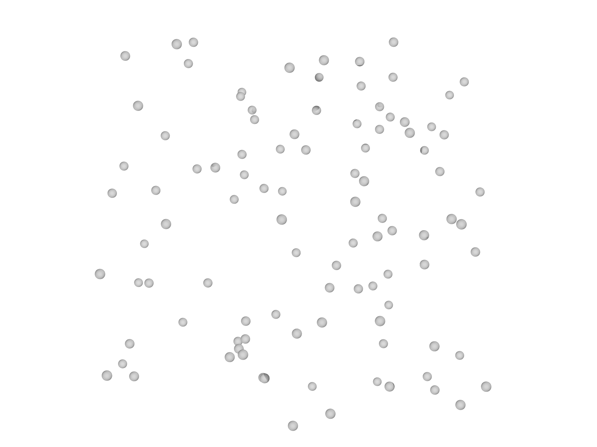
A major advantage of raytracing is natural support for transparency
effects. Here we generate 50 spheres of random placement, size and
transparency by setting the transmit option. The rendered output is
shown in Fig. 6.7.
fn randompt(R) {
    return R*Matrix([random()-1/2, random()-1/2, random()-1/2])
}

for (i in 1..50) {
    g.display(Sphere(randompt(1.5), random()/5, transmit=random()))
}
Examples
This chapter discusses the example programs provided to illustrate
various morpho features. These can be found in the examples folder
of the morpho git repository and are listed here in alphabetical order.
Some closely relate to material presented in other chapters for which
cross-references are provided.
Catenoid
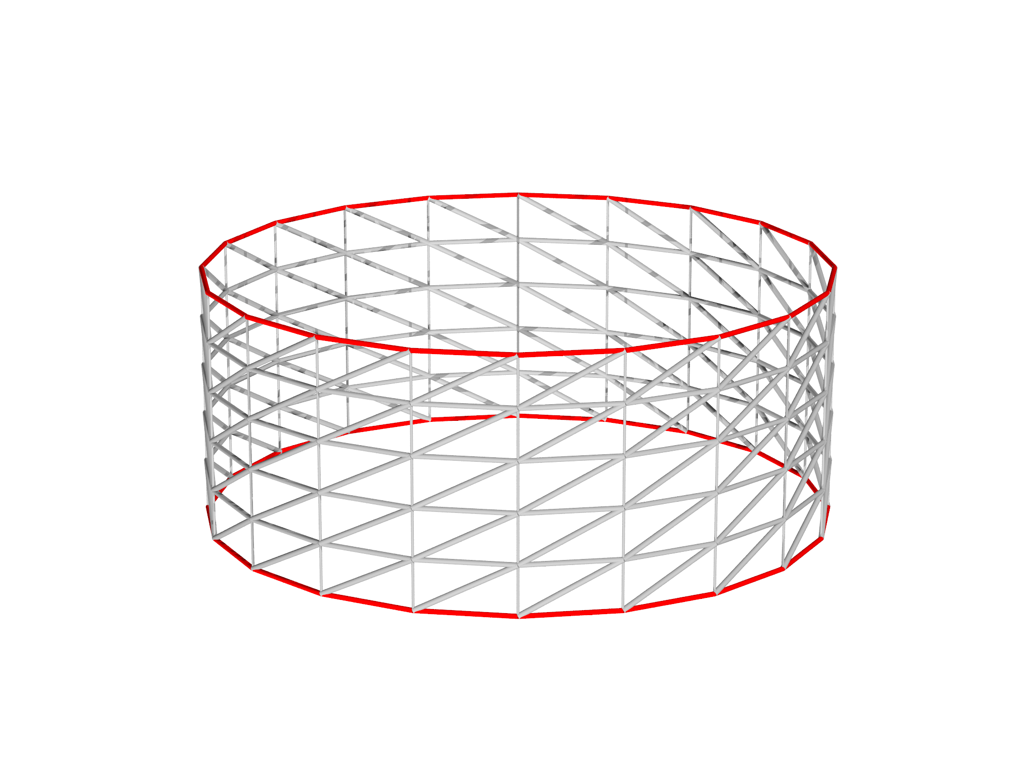

A soap film held between two parallel concentric circular rings adopts the shape of a minimal surface called a catenoid. This is a relatively simple optimization problem, and hence is a good example for beginners to morpho.
The initial mesh is created using AreaMesh in the meshtools module:
var r = 1.0 // radius
var ratio = 0.4 // Separation to diameter ratio
var L = 2*r*ratio // Separation

// Generate a tube / cylindrical mesh
var mesh = AreaMesh(fn (u, v) [r*cos(u), v, r*sin(u)],
                    -Pi...Pi:Pi/10,
                    -L/2..L/2:L/5,
                    closed=[true,false] )
mesh.addgrade(1)
The boundary of the mesh must be fixed in place. We can do this by creating a Selection, and visualizing it as shown in Fig. 7.1, left panel:
// Select the boundary
var bnd = Selection(mesh, boundary=true)
var g = plotselection(mesh, bnd, grade=1)
The optimization problem simply requires us to specify the area as the quantity to minimize:
 // Define the optimizataion problem
var problem = OptimizationProblem(mesh)
// Add the area energy using the built-in Area functional
var area = Area()
problem.addenergy(area)
We then create a ShapeOptimizer to perform the optimization,
var opt = ShapeOptimizer(problem, mesh)
fix the boundary elements using the selection object we created,
opt.fix(bnd)
and perform the optimization. Conjugate gradient works well for this problem and converges in a few iterations. The final optimized shape is shown in Fig. 7.1, right panel.
opt.conjugategradient(1000)
Cholesteric
A cholesteric liquid crystal, in contrast to a nematic liquid crystal as was considered in the tutorial in Chapter X, favors a twisted state. The liquid crystal elastic energy is modified to include a preferred chiral wavevector \(q_{0}\), $$ \begin{equation} F=\frac{1}{2}\int_{C}K_{11}\left(\nabla\cdot\mathbf{n}\right)^{2}+K_{22}(\mathbf{n}\cdot\nabla\times\mathbf{n}-q_{0})^{2}+K_{33}\left|\mathbf{n}\times\nabla\times\mathbf{n}\right|^{2}dA.\label{eq:CholestericFreeEnergy} \end{equation} $$ The cholesteric example minimizes the above equation in a square domain \((x,y)\in[-L,L]\), with \(L=1/2\), together with an anchoring energy, $$W\int(\mathbf{n}\cdot\mathbf{\hat{y}})^{2}dl,$$ imposed on the top and bottom boundaries to promote planar degenerate alignment, i.e. \(\mathbf{n}\) prefers to lie any direction in the \(x-z\) plane. The optimized structure with \(q_{0}=\pi/2\) is displayed in Fig. (7.2).
Cube
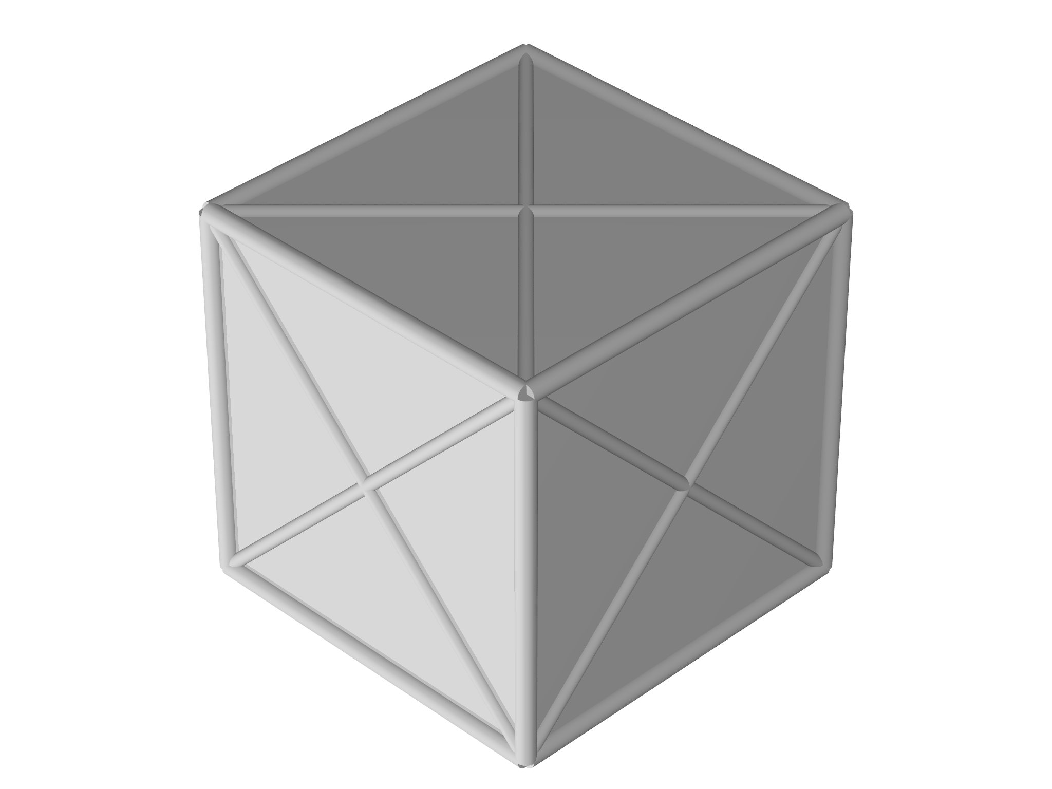

This example finds a minimal surface with fixed enclosed volume, i.e. a sphere. It closely parallels a similar example from Surface Evolver, and hence may aid those familiar with that program in learning to use morpho. Starting from an initial cube, shown in Fig. (7.3), and created as follows:
 // Create an initial cube
var m = PolyhedronMesh([ [-0.5, -0.5, -0.5],
                         [ 0.5, -0.5, -0.5],
                         [-0.5,  0.5, -0.5],
                         [ 0.5,  0.5, -0.5],
                         [-0.5, -0.5,  0.5],
                         [ 0.5, -0.5,  0.5],
                         [-0.5,  0.5,  0.5],
                         [ 0.5,  0.5,  0.5]],
                       [ [0,1,3,2], [4,5,7,6],
                         [0,1,5,4], [3,2,6,7],
                         [0,2,6,4], [1,3,7,5] ])
The problem and optimizer are set up:
var problem = OptimizationProblem(m)
var la = Area()
problem.addenergy(la)

var lv = VolumeEnclosed()
problem.addconstraint(lv)

var opt = ShapeOptimizer(problem, m)
The mesh is optimized, then refined, then reoptimized:
var Nlevels = 4 // Levels of refinement
var Nsteps = 1000 // Maximum number of steps per refinement level

for (i in 1..Nlevels) {
  opt.conjugategradient(Nsteps)
  if (i==Nlevels) break
  // Refine
  var mr=MeshRefiner([m])
  var refmap = mr.refine()
  for (el in [problem, opt]) el.update(refmap)
  m = refmap[m]
}
And finally the resulting area is compared with the true area of a sphere at the same volume:
var V0=lv.total(m)
var Af=la.total(m)
var R=(V0/(4/3*Pi))^(1/3)
var area = 4*Pi*R^2
print "Final area: ${Af} True area: ${area} diff: ${abs(Af-area)}"
Delaunay

This example demonstrates use of the delaunay module to create a
Delaunay triangulation from a point cloud. The triangulation generated
is explicitly checked for the property that no point other than the
vertices lies within the circumsphere of each triangle.
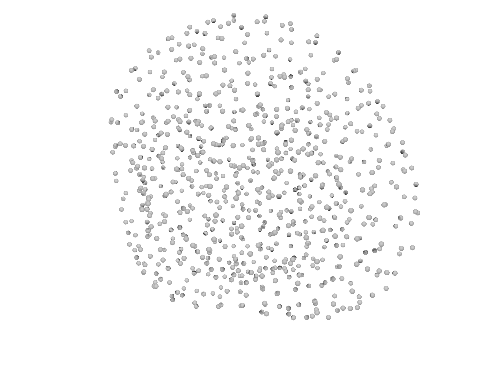
DLA
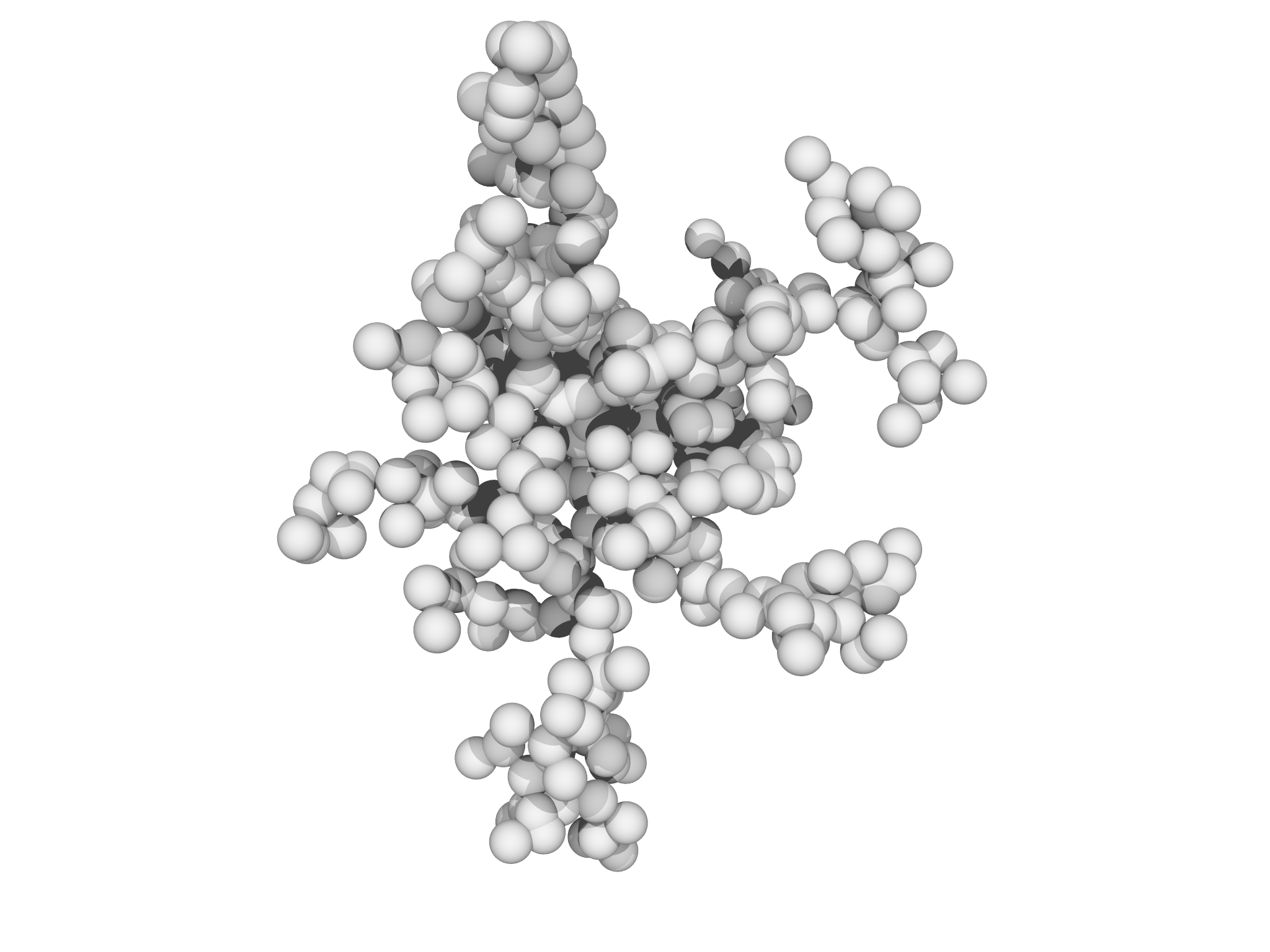
Diffusion Limited Aggregation is a process describing the formation of aggregates of sticky particles. An initial seed particle of radius \(r\) is placed at \( x_0=(0,0,0) \). Subsequent particles are added one by one from initial random points \(\mathbf{x}_{i}^{0}=R\mathbf{\xi}/|\mathbf{\xi}|\) where \(\xi\) is a random point normally distributed in each axis; the construction \(\mathbf{\xi}/|\mathbf{\xi}|\) generates a random point on the unit sphere. In morpho, this looks like
fn randompt() {
  var x = Matrix([randomnormal(), randomnormal(), randomnormal()])
  return R*x/x.norm()
}
The mobile particle moves diffusively, according to
$$ x_i^{n+1}=x_i^{n}+\delta\xi$$
where \(\delta\) is a small number. As the particle moves, we check to see if it has collided with any other particles, $$\left|x_{i}-x_{j}\right|<2r,\forall i\neq j,\label{eq:collisioncheck}$$ or if it has wandered out of bounds, $$\left|x_{i}\right|>2R.$$ If a particle has collided with another particle, it becomes fixed in place and joins the aggregate. As particles are added, the aggregate develops a characteristic fractalline morphology as shown in Fig. 7.5{reference-type="ref" reference="fig:DLA"}. The body of the program is a double loop:
for (n in 1..Np) { // Add particles one-by-one
  var x = randompt()
  while (true) {
    // Move current particle
    x+=Matrix([delta*randomnormal(), delta*randomnormal(), delta*randomnormal()])

    // Check for collisions
    /* ... */

    // Catch if it wandered out of the boundary
    if (x.norm()>2*R) x = randompt()
  }
}
To perform the collision check, the example uses a data structure called
a \(k\)-dimensional tree, provided in the kdtree module. A
\(k\)-dimensional tree provides a nearest neighbor search with \(O(\log N)\)
complexity rather than \(O(N)\) complexity as would be required by
searching all the points directly. The collision check code looks like
this:
if ((tree.nearest(x).location-x).norm()<2*r) {
  tree.insert(x)
  pts.append(x)
  if (x.norm()>R/2) R = 2*x.norm()
  break // Move to next particle
}
Notice that we gradually expand \(R\) as the aggregate grows. Ideally, each point should start very far away, really at infinity, but this would be very expensive in terms of the number of diffusion steps. A value of \(R\) double the greatest extent of the aggregate is a good compromise between speed and a reasonable approximation of diffusion limited aggregation.
This example also demonstrates how to create a simple custom
visualization directly using the graphics module. The particles are
drawn as spheres and displayed with the following code. An example run
is displayed in Fig. 7.5.
var col = Gray(0.5)
var g = Graphics()
g.background = White
for (x in pts) g.display(Sphere(x, r, color=col))
Show(g)
Electrostatics
This example shows how to solve a simple electrostatics problem with adaptive refinement, and provides a useful example of how to cast a problem that is normally thought of as solving a PDE as an optimization problem.
Suppose we want to solve Laplace's equation,
$$\nabla^{2}\phi=0$$
on a square domain \(C\) defined by \(-L/2\leq x\leq L/2\) and \(-L/2\leq y\leq L/2\). An equivalent formulation suitable for morpho is to minimize,
$$ \begin{equation} \int_{C}\left|\nabla\phi\right|^{2}dA \label{eq:el1} \end{equation} $$
with respect to \(\phi\).
We can show the two are equivalent by applying calculus of variations to the \eqref{eq:el1},
$$ \delta\int*{C}\left|\nabla\phi\right|^{2}dA =\int*{C}\delta\left|\nabla\phi\right|^{2}dA $$ $$ =\int_{C}\frac{\partial}{\partial\nabla\phi}\left|\nabla\phi\right|^{2}\cdot\delta\nabla\phi dA,$$
and integrating by parts,
$$ \begin{align} \int_{C}\frac{\partial}{\partial\nabla\phi}\left|\nabla\phi\right|^{2}\cdot\delta\nabla\phi dA & =\int_{\partial C}\nabla\phi\cdot\hat{\mathbf{s}}\delta\phi dl-\int_{C}\nabla\cdot\frac{\partial}{\partial\nabla\phi}\left|\nabla\phi\right|^{2}\delta\phi dA\nonumber \\ & =\int_{\partial C}\nabla\phi\cdot\hat{\mathbf{s}}\delta\phi dl-\int_{C}\nabla^{2}\phi\delta\phi dA,\label{eq:bulkvariations} \end{align} $$
Note If you're not familiar with calculus of variations, feel free to skip paragraphs that refer to "variations". The calculus of variations generalizes calculus from differentiating with respect to variables to differentiating with respect to functions.
where \(\hat{\mathbf{s}}\) is the outward normal. Hence, allowing for arbitrary variations \(\delta\phi\), in order for the bulk integrand to vanish Laplace's equation \(\nabla^{2}\phi=0\) must be satisfied. Similarly requiring the boundary integrand to vanish yields the "natural" boundary condition \(\nabla\phi\cdot\hat{\mathbf{s}}=0\), known as the Neumann boundary condition. In the absence of boundary energies, solving \(\nabla^{2}\phi=0\) in \(C\) subject to \(\nabla\phi\cdot\hat{\mathbf{s}}=0\) on \(\partial C\) yields the family of uniform constant solutions \(\phi=\text{const}.\)
To impose boundary data, we will supplement \eqref{eq:el1} with the additional functional,
$$ \begin{equation} \lambda\int_{\partial C}\left[\phi-\phi_{0}(\mathbf{x})\right]^{2}dl\label{eq:anchoring} \end{equation} $$
where the function \(\phi_{0}\) represents some imposed boundary potential. Taking variations of this functional,
$$ \begin{align} \delta\lambda\int_{\partial C}\left[\phi-\phi_{0}(\mathbf{x})\right]^{2}dl & =\lambda\int_{\partial C}\frac{\partial}{\partial\phi}\left[\phi-\phi_{0}(\mathbf{x})\right]^{2}\delta\phi dl\nonumber \\ & =\lambda\int_{\partial C}2\left[\phi-\phi_{0}(\mathbf{x})\right]\delta\phi dl\label{eq:boundary} \end{align} $$
Collecting the boundary terms from \eqref{eq:bulkvariations} and \eqref{eq:boundary}, we obtain the equivalent boundary condition on \(\phi\), $$\nabla\phi\cdot\hat{\mathbf{s}}+2\lambda(\phi-\phi_{0})=0,$$ which is known as a Robin boundary condition. As \(\lambda\to\infty\), \(\phi\to\phi_0\) on the boundary, recovering a fixed boundary or Dirichlet condition, while as \(\lambda\to0\), we recover the Neumann conditions discussed earlier.
In the example, we will set \(\phi_0=0\) on the left and lower boundary and \(\phi_0=1\) on the right and upper boundary, and use \(\lambda=100\).
The code illustrates a few morpho tricks. First, the following code is used to select the left/bottom and upper/right sides of the mesh:
var bnd = Selection(mesh, boundary=true)
var bnd1 = Selection(mesh, fn (x,y,z) abs(x+L/2)<0.01 || abs(y+L/2)<0.01)
var bnd2 = Selection(mesh, fn (x,y,z) abs(x-L/2)<0.01 || abs(y-L/2)<0.01)
for (b in [bnd1, bnd2]) b.addgrade(1)
bnd1=bnd.intersection(bnd1)
bnd2=bnd.intersection(bnd2)
What's happening here is that we select the whole boundary in the first
line and then select relevant vertices in the next two lines. The edges
are then added to the selection with addgrade, but this also selects
some interior edges. To ensure we only have boundary edges in our
selections, we find the intersection of bnd1 and bnd, and similarly
for bnd2.
The problem setup involves adding the electrostatic energy Eq.\eqref{eq:el1} using
GradSq and the boundary terms Eq.\eqref{eq:anchoring} as LineIntegrals.
var problem = OptimizationProblem(mesh)
var le = GradSq(phi)
problem.addenergy(le)
var v1 = 0, v2 = 1
var lt1 = LineIntegral(fn (x, v) (v-v1)^2, phi)
problem.addenergy(lt1, selection=bnd1, prefactor=100)
var lt2 = LineIntegral(fn (x, v) (v-v2)^2, phi)
problem.addenergy(lt2, selection=bnd2, prefactor=100)
Optimization is done with a FieldOptimizer:
var opt = FieldOptimizer(problem, phi)
opt.conjugategradient(100)
The problem as posed requires \(\phi\) to very sharply change in the upper left and lower right cornes as the imposed potential changes, but far away from these \(\phi\) changes much more slowly. We would like therefore to perform adaptive refinement, refining the mesh only in places where \(\phi\) is rapidly changing and using coarse elements elsewhere.
To identify elements to refine, we compute the electrostatic energy in each elementwe'll use this as a heuristic measure of how rapidly \(\phi\) is changingand find the mean energy per element. We then create a Selection and manually select elements that have an electrostatic energy more than \(1.5\times\) the mean.
// Select elements that have an above average contribution to the energy
var en = le.integrand(phi) // energy in each element
var mean = en.sum()/en.count() // mean energy per element
var srefine = Selection(mesh)
for (id in 0...en.count()) if (en[0,id]>1.5*mean) srefine[2,id]=true
// identify large contributions
Refinement is then performed with a MeshRefiner object from the
meshtools module, which we create with a list of both the mesh to
refine and all quantities that refer to the mesh:
var ref = MeshRefiner([mesh, phi, bnd, bnd1, bnd2])
The refinement is performed using the selection srefine just created
var refmap = ref.refine(selection=srefine)
which returns a Dictionary mapping the old quantities to the new refined ones. We use this dictionary to update the OptimizationProblem and FieldOptimizer,
for (el in [problem, opt]) el.update(refmap)
and finally update our variables
mesh = refmap[mesh]
phi = refmap[phi]
bnd = refmap[bnd]
bnd1 = refmap[bnd1]
bnd2 = refmap[bnd2]
Finally, we equiangulate the mesh to help avoid narrow elements,
equiangulate(mesh)
Once refinement is complete, further optimization can occur on the newly refined mesh
opt.conjugategradient(1000)
The process of refinement and optimization just described takes place in a loop. The resulting mesh after 10 iterations is shown in Fig. 7.6, together with the solution \(\phi\). The code runs in a few seconds, providing a considerable speedup over optimizing on a fine grid to get comparable accuracy.


Implicitmesh
These examples illustrate how to use the implicitmesh module to
generate surfaces described as the zero set of a scalar function. The
sphere.morpho and torus.morpho examples are described more fully in
Chapter X, Section Y. The remaining threesurface.morpho creates a
triangulation of a surface with three handles,
$$r_{z}^{4}z^{2}-\left(1-\left(\frac{x}{r_{x}}\right)^{2}-\left(\frac{y}{r_{y}}\right)^{2}\right)\left((x-x_{1})^{2}+y^{2}-r_{1}^{2}\right)\left((x+x_{1})^{2}+y^{2}-r_{1}^{2}\right)\left(x^{2}+y^{2}-r_{1}^{2}\right)=0,$$
where \(r_{x}\), \(r_{y}\), \(r_{z}\), \(r_{1}\) and \(x_{1}\) are parameters. The
resulting surface is shown in Fig.
7.7.
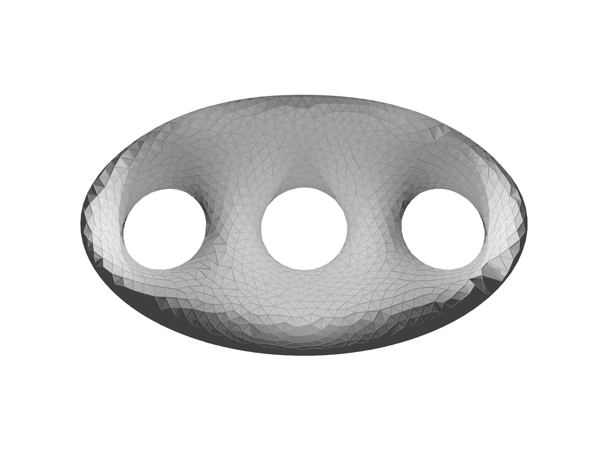
implicitmesh
module.Meshgen
Examples in this folder illustrate various techniques to create Meshes
with the meshgen module. Examples in two dimensions are shown in Fig.
7.8;
those in 3D are shown in Fig. 7.9. See also the Meshgen Section of the Working with Meshes Chapter for
additional discussion of the meshgen module.
A B
B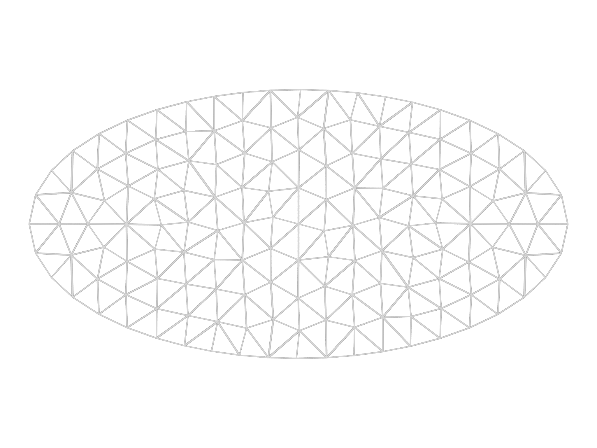
C D
D
E F
F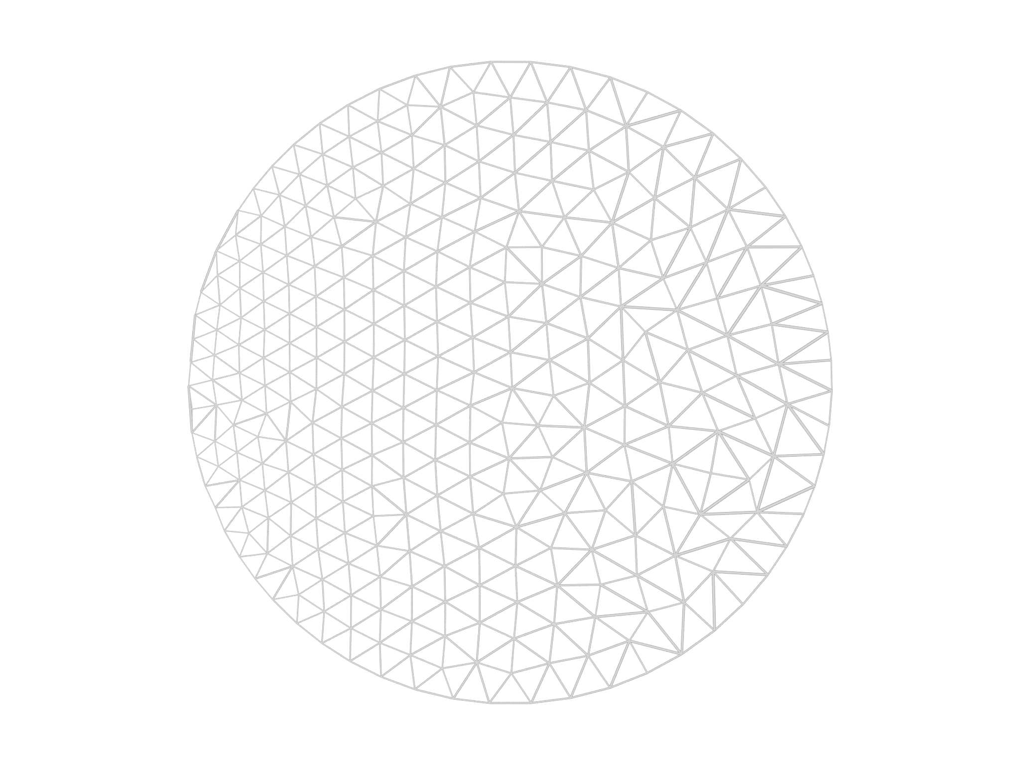
meshgen
module. A disk.morpho,
B ellipse.morpho, C
halfdisk.morpho, D
overlappingdisks.morpho, E
superellipse.morpho, F
weighted.morphoA B
B
C
meshgen
module. A sphere.morpho,
B ellipsoidsection.morpho,
C superellipsoid.morpho.Meshslice
This example shows how to use the meshslice module to create a slice
through a mesh for visualization purposes. The program uses a spherical
mesh,
var m = Mesh("sphere.mesh")
m.addgrade(1)
m.addgrade(2)
and creates a couple of example Fields, one scalar,
var phi = Field(m, fn (x,y,z) x+y+z)
and one vector,
var nn = Field(m, fn (x,y,z) Matrix([x,y,z])/sqrt(x^2+y^2+z^2))
A MeshSlicer is created to do the slicing,
var slice = MeshSlicer(m)
var slc = slice.slice([0,0,0], [1,0,0])
and then interpolated Fields along this slice are created too,
var sphi = slice.slicefield(phi)
var snn = slice.slicefield(nn)
Grade 1 elements (edges) from the original mesh, together with the field phi interpolated onto three different slices, are shown in Fig. 7.10. The example program illustrates a few other different possibilities.
Plot
This example illustrates drawing of meshes, plotting of fields, etc. See the Visualization Chapter for more details.
Povray
Examples in this folder illustrates use of the povray module used to
produce publication quality renderings from within morpho programs.
All figures in this book were generated using this module.
Qtensor
This example demonstrates use of the alternative Q-tensor formulation of nematic liquid crystal theory. We briefly present the necessary theory in two subsections below, then describe the implementation in morpho.
The Q tensor
In 2D, for a uniaxial nematic, we can define a Q-tensor: $$Q_{ij}=S(n_{i}n_{j}-1/2\delta_{ij})$$ Here, the \(-1/2\delta_{ij}\) is added for convenience, to make the matrix traceless: $$\text{Tr}(\mathbf{Q})=Q_{ii}=S(n_{i}n_{i}-1/2\delta_{ii})=S(1-1/2(2))=0$$ Now, the Q-tensor is also symmetric by definition: $$Q_{ij}=Q_{ji}$$ Due to these two reasons we can write the Q-tensor as a function of only \(Q_{xx}\) and \(Q_{xy}\):
$$ \mathbf{Q}= \begin{bmatrix} Q_{xx} & Q_{xy} \\ Q_{xy} & -Q_{xx} \end{bmatrix}. $$
Elastic Energy and Anchoring
The Landau-de Gennes equilibrium free energy for a nematic liquid crystal can be written in terms of the Q-tensor:
$$ F_{LDG}= \int_{\Omega}d^{2}{\bf x}\ \left(\frac{a_{2}}{2}\text{Tr}(\mathbf{Q}^{2})+\frac{a_{4}}{4}(\text{Tr}\mathbf{Q}^{2})^{2}+\frac{K}{2}(\nabla\mathbf{Q})^{2}\right) $$ $$ +\oint_{\partial\Omega}d{\bf x}\frac{1}{2}E_{A}\text{Tr}[(\mathbf{Q}-\mathbf{W})^{2}] $$
where \(a_{2}=(\rho-1)\) and \(a_{4}=(\rho+1)/\rho^{2}\) set the isotropic to nematic transition with \(\rho\) being the non-dimensional density. The system is in the isotropic state for \(\rho<1\) and in the nematic phase when \(\rho>1\). In the nematic phase, \(\ell_{n}=\sqrt{K/a_{2}}\) sets the nematic coherence length. Now,
$$\mathbf{Q}^{2}=\begin{bmatrix}Q_{xx} & Q_{xy} \\ Q_{xy} & -Q_{xx} \end{bmatrix}\begin{bmatrix}Q_{xx} & Q_{xy} \\ Q_{xy} & -Q_{xx} \end{bmatrix}=(Q_{xx}^{2}+Q_{xy}^{2})\begin{bmatrix}1 & 0 \\ 0 & 1 \end{bmatrix}$$ Hence, $$\text{Tr}(\mathbf{Q}^{2})=2(Q_{xx}^{2}+Q_{xy}^{2})$$ Similarly, $$(\nabla\mathbf{Q})^{2}=\partial_{i}Q_{kj}\partial_{i}Q_{kj}=2{(\partial_{x}Q_{xx})^{2}+(\partial_{x}Q_{xy})^{2}+(\partial_{y}Q_{xx})^{2}+(\partial_{y}Q_{xy})^{2}}$$ Now, the second term is a boundary integral, with \(E_{A}\) being the anchoring strength. \(\mathbf{W}\) is the tensor corresponding to the boundary condition. For instance, for parallel anchoring, $$W_{ij}=(t_{i}t_{j}-1/2\delta_{ij})$$ where \(t_{i}\) is a component of the tangent vector at the boundary. \(\mathbf{W}\) is also a symmetric traceless tensor with two independent components \(W_{xx}\) and \(W_{xy}\). The boundary term becomes: $$\text{Tr}[(\mathbf{Q}-\mathbf{W})^{2}]=2{Q_{xx}^{2}+Q_{xy}^{2}-2(Q_{xx}W_{xx}+Q_{xy}W_{xy})+W_{xx}^{2}+W_{xy}^{2}}$$
Optimization problem
We can formulate all the preceding expressions in terms of vector quantities: $$\vec{q}\equiv \{ Q_{xx},Q_{xy} \} $$ $$\vec{w}\equiv \{w_{xx},w_{xy} \}$$ Thus, $$\text{Tr}(\mathbf{Q}^{2})=2||\vec{q}||^{2}$$
$$(\nabla\mathbf{Q})^{2}=2||\nabla\vec{q}||^{2}$$
$$\text{Tr}[(\mathbf{Q}-\mathbf{W})^{2}]=2||\vec{q}-\vec{w}||^{2}$$ With these, we want to minimize the area-integral of $$F=\int_{\Omega}d^{2}{\bf x}\ \left(a_{2}||\vec{q}||^{2}+a_{4}||\vec{q}||^{4}+K||\nabla\vec{q}||^{2}\right)$$ together with the line-integral energy $$\oint_{\partial\Omega}d{\bf x}\ E_{A}||\vec{q}-\vec{w}||^{2}$$
Implementation
This free energy is readily set up in morpho. For this example, we consider a 2D disk geometry with unit radius. We use \(\rho=1.3\), so that we are deep in the nematic regime. We fix \(E_{\text{A}}=3\), which sets strong anchoring at the boundary. With this strong tangential anchoring, we get a topological charge of \(+1\) at the boundary, and this acts as a constraint. When the nematic coherence length is comparable to the disk diameter (\(\ell_{n}\sim R\)), the \(+1\) charge penetrates throughout the disk, whereas if (\(\ell_{n}\ll R\)), then a formation with 2 \(+1/2\) defects is more stable. To test this, we use two different values of \(K\):, 0.01 and 1.0.
We first define all our parameters and import \(\texttt{disk.mesh}\) from the tactoid example:
var rho = 1.3 // Deep in the nematic phase
var EA = 3 // Anchoring strength
var K = 0.01 // Bending modulus

var a2 = (1-rho)
var a4 = (1+rho)/rho^2

var m = Mesh("disk.mesh")
var m = refinemesh(m) // Refining for a better result
var bnd = Selection(m, boundary=true)
bnd.addgrade(0) // add point elements
We define the Q-tensor in its vector form as discussed above, initializing it to small random values:
var q_tensor = Field(m, fn(x,y,z)
Matrix([0.01*random(1), 0.01*random(1)]))
Note that this incidentally makes the director parallel to a 45 degree line. We now define the bulk energy, the anchoring energy and the distortion free energy as follows:
// Define bulk free energy
fn landau(x, q) {
  var qt = q.norm()
  var qt2=qt*qt
  return a2*qt2 + a4*qt2*qt2
}
// Define anchoring energy at the boundary
fn anchoring(x, q) {
  var t = tangent()
  var wxx = t[0]*t[0]-0.5
  var wxy = t[0]*t[1]
  return (q[0]-wxx)^2+(q[1]-wxy)^2
}

var bulk = AreaIntegral(landau, q_tensor)
var anchor = LineIntegral(anchoring, q_tensor)
var elastic = GradSq(q_tensor)
Equipped with the energies, we define the OptimizationProblem:
var problem = OptimizationProblem(m)
problem.addenergy(bulk)
problem.addenergy(elastic, prefactor = K)
problem.addenergy(anchor, selection=bnd, prefactor=EA)
To minimize the energy with respect to the field, we define the
FieldOptimizer and perform a linesearch:
var opt = FieldOptimizer(problem, q_tensor)
opt.linesearch(500)
Visualization
For visualizing the final configuration, we use the same piece of code we used for the tactoid example, and define some additional helper functions to extract the director and the order from the Q-tensor:
fn qtodirector(q) {
  var S = 2*q.norm()
  var Q = q/S
  var nx = sqrt(Q[0]+0.5)
  var ny = abs(Q[1]/nx)
  nx*=sign(Q[1])
  return Matrix([nx,ny,0])
}

fn qtoorder(q) {
  var S = 2*q.norm()
  return S
}
We use these to create Fields from q_tensor.
// Convert the q-tensor to the director and order
var nn = Field(m, Matrix([1,0,0]))
for (i in 0...m.count()) nn[i]=qtodirector(q_tensor[i])
var S = Field(m, 0)
for (i in 0...m.count()) S[i]=qtoorder(q_tensor[i])
and display these, reusing the visualize function from the tactoid
tutorial example.
var splot = plotfield(S, style="interpolate")
var gnn=visualize(m, nn, 0.05)
var gdisp = splot+gnn
Show(gdisp)
This creates beautiful plots of the nematic, displayed in Fig. 7.11. Like the tactoid example, we can do adaptive mesh refinement based on the elastic energy density as well.
Thomson
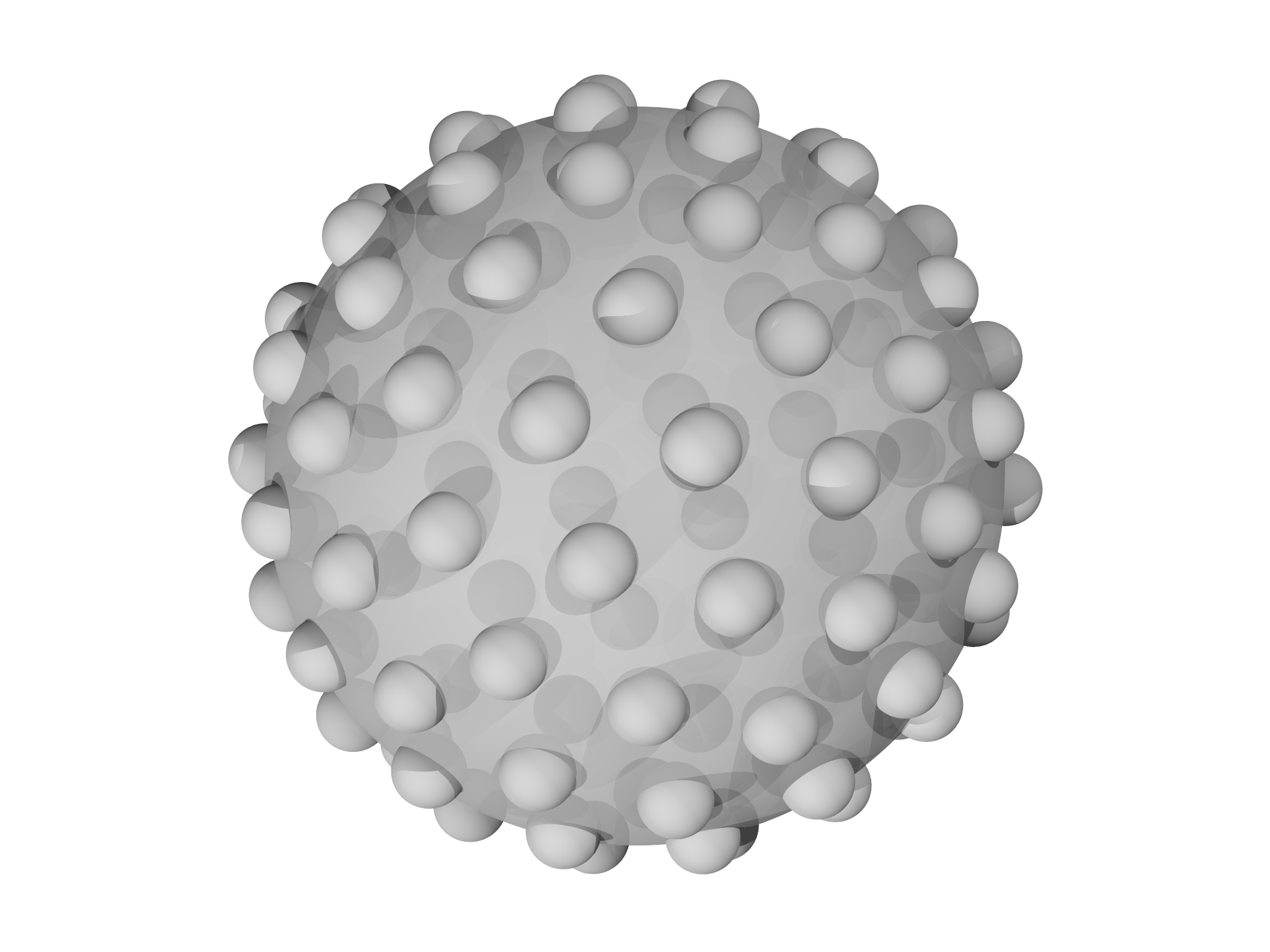
Consider \(N\) charges \(q\) with positions \(x_i\) that are each confined to lie on the unit sphere so that \(\left| x_i\right|=1 \) that repel each other electrostatically and hence whose configuration minimizes the energy, $$\frac{k}{2}\sum_{i\neq j}\frac{q^{2}}{\left|x_{i}-x_{j}\right|}$$ The problem was posed by the physicist J. J. Thomson in 1904, in the context of an early model for the structure of an atom.
To set this up in morpho, we begin by creating a mesh from a sequence
of random points using a MeshBuilder object from the meshtools module.
Notice that this is quite an unusual mesh; it consists of \(N\)
unconnected points with no connectivity information.
var build = MeshBuilder()
for (i in 1..Np) {
  var x = Matrix([2*random()-1, 2*random()-1, 2*random()-1])
  x/=x.norm() // Project onto unit sphere
  build.addvertex(x)
}
var mesh = build.build()
The optimization problem is then specified. We use the PairwisePotential
functional from the functionals module and supply the Coulomb
potential \(1/r\), together with its derivative \(-1/r^{2}\) as anonymous
functions:
var problem = OptimizationProblem(mesh)
var lv = PairwisePotential(fn (r) 1/r, fn (r) -1/r^2)
problem.addenergy(lv)
Constraining the particles to a sphere is implemented as a level set constraint: We use the ScalarPotential functional as a local constraint to ensure that each particle lies on the zero contour of the scalar function \(x^{2}+y^{2}+z^{2}-1\), which defines the unit sphere.
var lsph = ScalarPotential(fn (x,y,z) x^2+y^2+z^2-1) problem.addlocalconstraint(lsph)
Optimization is then performed:
var opt = ShapeOptimizer(problem, mesh)
opt.stepsize=0.01/sqrt(Np)
opt.relax(5)
opt.conjugategradient(1000)
Notice that we estimate the initial stepsize from the number of
particles. Since each particle will adopt a fraction \(1/N\) of the area,
the stepsize is \(\propto1/\sqrt{N}\). In practice, we find that taking a
few steps of gradient descent with relax helps condition the problem by
pushing any particles from the initially random distribution that
happened to be placed very close to one another apart. After this
conjugategradientworks well and typically converges in around \(100\)
iterations.
A final interesting feature of this example is the use of a custom visualization. We draw a sphere with a center of mass at the location at each particle:
var g = Graphics()
for (i in 0...mesh.count()) {
  g.display(Sphere(mesh.vertexposition(i),1/sqrt(Np)))
}
g.display(Sphere([0,0,0],1))
Show(g)
A typical configuration resulting from this is shown in Fig.
7.12. Note
that we made the large sphere transparent to render with the povray
module; this was achieved by adding the optional argument transmit=0.3
to the call to Sphere.
Wrap
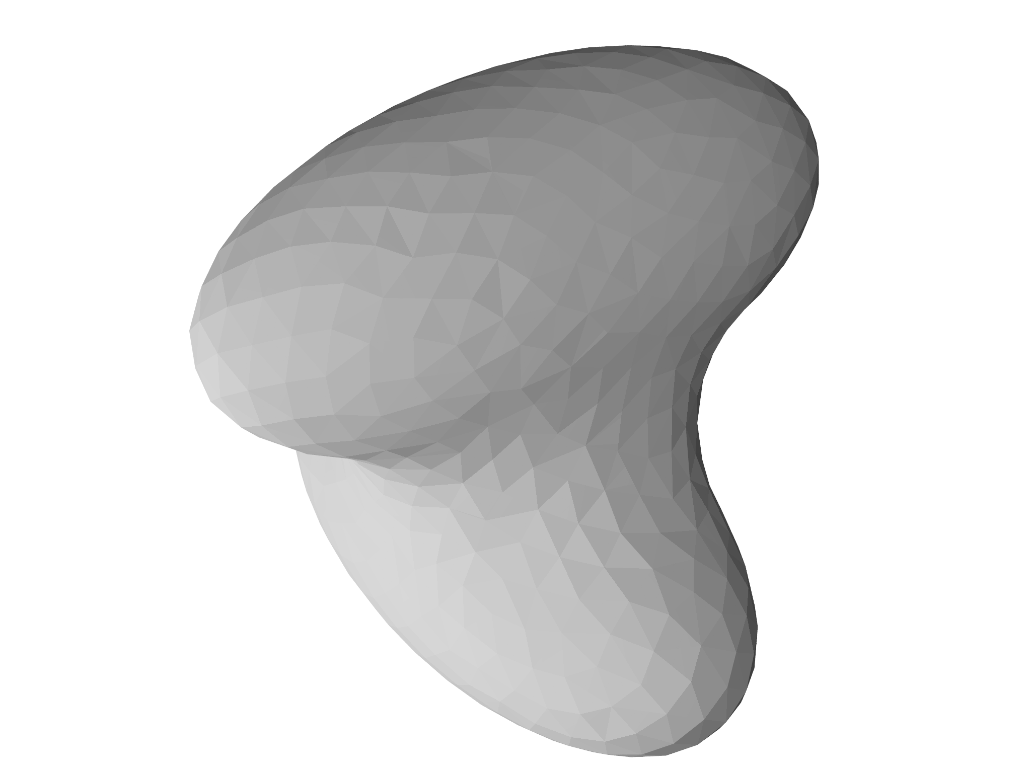
The wrap example finds a minimal surface constrainted to lie outside two ellipsoids. The solution, shown in Fig. 7.13 could represent, for example, a possible configuration for a fluid bridge connecting two ellipsoidal particles.
The basic idea of this code is to "shrink wrap" the ellipsoids, starting
with an initial mesh is a cube that completely encloses them. This is
created with PolyhedronMesh from the meshtools module:
// Create a initial cube
var L = 2
var cube = [[-L, -L, -L], [-L, -L, L], [-L, L, -L],
            [-L, L, L], [L, -L, -L], [L, -L, L],
            [L, L, -L], [L, L, L]]

var faces = [[7, 3, 1, 5], [7, 5, 4, 6], [7, 6, 2, 3], [3, 2, 0, 1], [0, 2, 6,   4], [1, 0, 4, 5]]

var m=PolyhedronMesh(cube, faces)
m=refinemesh(m)
The particles are implemented as level set constraints. A convenient Ellipsoid class is defined to help create appropriate constraints,
class Ellipsoid { // Construct with Ellipsoid(origin, principalradii)
  init(x, r) {
    self.origin = x
    self.principalradii = r
  }
  // Returns a level set function for this Ellipsoid
  levelset() {
    fn phi (x,y,z) {
      var x0 = self.origin, rr = self.principalradii
      return ((x-x0[0])/rr[0])^2 + ((y-x0[1])/rr[1])^2 + ((z-x0[2])/rr[2])^2 - 1
    }
    return phi
  }
  /* Analogous code for gradient() ... */
}
The levelset method manufactures a scalar function representing the
ellipsoid and suitable for use with the ScalarPotential functional. A
second method, gradient, returns the gradient of that function.
The two ellipsoids of interest are then created like so:
var ell1 = Ellipsoid([0,1/2,0],[1/2,1/2,1])
var ell2 = Ellipsoid([0,-1/2,0],[1,1/2,1/2])
The optimization problem is set up to include the surface area subject to satisfaction of the level set constraints; these are noted as one-sided, i.e. satisfied if the mesh lies at any point outside the constraint region.
// We want to minimize the area
var la = Area() // Subject to level set constraints
var ls1 = ScalarPotential( ell1.levelset(), ell1.gradient() )
var ls2 = ScalarPotential( ell2.levelset(), ell2.gradient() )
var leq = EquiElement()

var problem = OptimizationProblem(m)
problem.addenergy(la)
problem.addlocalconstraint(ls1, onesided=true)
problem.addlocalconstraint(ls2, onesided=true)
To promote mesh quality, a second regularization problem is set up:
var reg = OptimizationProblem(m)
reg.addenergy(leq)
reg.addlocalconstraint(ls1, onesided=true)
reg.addlocalconstraint(ls2, onesided=true)
Optimization and refinement are performed iteratively:
sopt.stepsize=0.025
sopt.steplimit=0.1
ropt.stepsize=0.01
ropt.steplimit=0.2
for (refine in 1..3) {
  for (i in 1..100) {
    sopt.relax(5)
    ropt.conjugategradient(1)
    equiangulate(m)
  }
  var mr=MeshRefiner([m])
  var refmap = mr.refine()
  for (el in [problem, reg, sopt, ropt]) el.update(refmap)
  m = refmap[m]
}
Note that we set stepsize and steplimit on each optimizer; these
values were found by trial and error. The initial shape is quite
extreme, and so we use relax for the main optimization problem which
is very robust. Calling equiangulate helps maintain mesh quality.
Reference
This chapter mirrors the documentation of everything shipped with the core Morpho distribution. The documentation is organized in the following sections:
The Language section provides a detailed description of the Morpho language, including the syntax and semantics of the language.
The Data Types section describes the various data types like List's, Matrix objects, etc.
The Computational Geometry section provides the documentation for meshes, selections, fields and functionals.
The I/O section provides the documentation for the File object.
The Modules section provides the documentation for the various standard modules shipped with Morpho.
Language
This section provides a detailed description of the Morpho language, including the syntax and semantics of the language.
Syntax
Morpho provides a flexible object oriented language similar to other languages in the C family (like C++, Java and Javascript) with a simplified syntax.
Morpho programs are stored as plain text with the .morpho file extension. A program can be run from the command line by typing
morpho5 program.morpho
Comments
Two types of comment are available. The first type is called a 'line comment' whereby text after // on the same line is ignored by the interpreter.
a.dosomething() // A comment
Longer 'block' comments can be created by placing text between /* and */. Newlines are ignored
/* This
   is
   a longer comment */
In contrast to C, these comments can be nested
/* A nested /* comment */ */
enabling the programmer to quickly comment out a section of code.
Symbols
Symbols are used to refer to named entities, including variables, classes, functions etc. Symbols must begin with a letter or underscore _ as the first character and may include letters or numbers as the remainder. Symbols are case sensitive.
asymbol
_alsoasymbol
another_symbol
EvenThis123
YET_ANOTHER_SYMBOL
Classes are typically given names with an initial capital letter. Variable names are usually all lower case.
Newlines
Strictly, morpho ends statements with semicolons like C, but in practice these are usually optional and you can just start a new line instead. For example, instead of
var a = 1; // The ; is optional
you can simply use
var a = 1
If you want to put several statements on the same line, you can separate them with semicolons:
var a = 1; print a
There are a few edge cases to be aware of: The morpho parser works by accepting a newline anywhere it expects to find a semicolon. To split a statement over multiple lines, signal to morpho that you plan to continue by leaving the statement unfinished. Hence, do this:
print a +
      1
rather than this:
print a   // < Morpho thinks this is a complete statement
      + 1 // < and so this line will cause a syntax error
Booleans
Comparison operations like ==, < and >= return true or false depending on the result of the comparison. For example,
print 1==2
prints false. The constants true or false are provided for you to use in your own code:
return true
Nil
The keyword nil is used to represent the absence of an object or value.
Note that in if statements, a value of nil is treated like false.
if (nil) {
    // Never executed.
}
Blocks
Code is divided into blocks, which are delimited by curly brackets like this:
{
  var a = "Hello"
  print a
}
This syntax is used in function declarations, loops and conditional statements.
Any variables declared within a block become local to that block, and cannot be seen outside of it. For example,
var a = "Foo"
{
  var a = "Bar"
  print a
}
print a
would print "Bar" then "Foo"; the version of a inside the code block is said to shadow the outer version.
Precedence
Precedence refers to the order in which morpho evaluates operations. For example,
print 1+2*3
prints 7 because 2*3 is evaluated before the addition; the operator * is said to have higher precedence than +.
You can always modify the order of evaluation by using parentheses:
print (1+2)*3 // prints 9
The print keyword is used to print information to the console. It can be followed by any value, e.g.
print 1
print true
print a
print "Hello"
Values
Values are the basic unit of information in morpho: All functions in morpho accept values as arguments and return values.
Int
Morpho provides integers, which work as you would expect in other languages, although you rarely need to worry about the distinction between floats and integers.
Convert a floating point number to an Integer:
print Int(1.3) // expect: 1
Convert a string to an integer:
print Int("10")+1 // expect: 11
Float
Morpho provides double precision floating point numbers.
Convert a string to a floating point number:
print Float("1.2e2")+1 // expect: 121
Ceil
Returns the smallest integer larger than or equal to its argument:
print ceil(1.3) // expect: 2
Floor
Returns the largest integer smaller than or equal to its argument:
print floor(1.3) // expect: 1
Format
The format method converts a number to a String using a given format specifier:
print (1/3).format("%4.2g") // Outputs 0.33
The specifier must begin with '%' and may include:
- A minimum width, given as an integer.
- Number of decimal places to show, with '.' in front.
- A formatting option, either 'f' or 'g' where:
- 'f' displays the number in decimal form, e.g. 0.01
- 'g' uses scientific notation, e.g. 1e-2
The syntax for the formatting string is similar to that used in C and Python.
Variables
Variables are defined using the var keyword followed by the variable name:
var a
Optionally, an initial assignment may be given:
var a = 1
Variables defined in a block of code are visible only within that block, so
var greeting = "Hello"
{
    var greeting = "Goodbye"
    print greeting
}
print greeting
will print
Goodbye Hello
Multiple variables can be defined at once by separating them with commas
var a, b=2, c[2]=[1,2]
where each can have its own initializer (or not).
Indexing
Morpho provides a number of collection objects, such as List, Range, Array, Dictionary, Matrix and Sparse, that can contain more than one value. Index notation (sometimes called subscript notation) is used to access elements of these objects.
To retrieve an item from a collection, you use the [ and ] brackets like this:
var a = List("Apple", "Bag", "Cat")
print a[0]
which prints Apple. Note that the first element is accessed with 0 not 1.
Similarly, to set an entry in a collection, use:
a[0]="Adder"
which would replaces the first element in a with "Adder".
Some collection objects need more than one index,
var a = Matrix([[1,0],[0,1]])
print a[0,0]
and others such as Dictionary use non-numerical indices,
var b = Dictionary()
b["Massachusetts"]="Boston"
b["California"]="Sacramento"
as in this dictionary of state capitals.
Control Flow
Control flow statements are used to determine whether and how many times a selected piece of code is executed. These include:
if- Selectively execute a piece of code if a condition is met.else- Execute a different block of code if the test in anifstatement fails.for- Repeatedly execute a section of code with a counterwhile- Repeatedly execute a section of code while a condition is true.
If
If allows you to selectively execute a section of code depending on whether a condition is met. The simplest version looks like this:
if (x<1) print x
where the body of the loop, print x, is only executed if x is less than 1. The body can be a code block to accommodate longer sections of code:
if (x<1) {
    ... // do something
}
If you want to choose between two alternatives, use else:
if (a==b) {
    // do something
} else {
    // this code is executed only if the condition is false
}
You can even chain multiple tests together like this:
if (a==b) {
    // option 1
} else if (a==c) {
    // option 2
} else {
    // something else
}
While
While loops repeat a section of code while a condition is true. For example,
var k=1
while (k <= 4) { print k; k+=1 }
       ^cond   ^body
prints the numbers 1 to 4. The loop has two sections: cond is the condition to be executed and body is the section of code to be repeated.
Simple loops like the above example, especially those that involve counting out a sequence of numbers, are more conveniently written using a for loop,
for (k in 1..4) print k
Where while loops can be very useful is where the state of an object is being changed in the loop, e.g.
var a = List(1,2,3,4)
while (a.count()>0) print a.pop()
which prints 4,3,2,1.
Do
A do...while loop repeats code while a condition is true---similar to a while loop---but the test happens at the end:
var k=1
do {
  print k;
  k+=1
} while (k<5)
which prints 1,2,3,4
Hence this type of loop executes at least one interation
For
For loops allow you to repeatedly execute a section of code. They come in two versions: the simpler version looks like this,
for (var i in 1..5) print i
which prints the numbers 1 to 5 in turn. The variable i is the loop variable, which takes on a different value each iteration. 1..5 is a range, which denotes a sequence of numbers. The body of the loop, print i, is the code to be repeatedly executed.
Morpho will implicitly insert a var before the loop variable if it's missing, so this works too:
for (i in 1..5) print i
If you want your loop variable to count in increments other than 1, you can specify a stepsize in the range:
for (i in 1..5:2) print i
               ^step
Ranges need not be integer:
for (i in 0.1..0.5:0.1) print i
You can also replace the range with other kinds of collection object to loop over their contents:
var a = Matrix([1,2,3,4])
for (x in a) print x
Morpho iterates over the collection object using an integer counter variable that's normally hidden. If you want to know the current value of the counter (e.g. to get the index of an element as well as its value), you can use the following:
var a = [1, 2, 3]
for (x, i in a) print "${i}: ${x}"
Morpho also provides a second form of for loop similar to that in C:
for (var i=0; i<5; i+=1) { print i }
     ^start   ^test ^inc.  ^body
which is executed as follows:
start: the variable i is declared and initially set to zero.
test: before each iteration, the test is evaluated. If the test is false, the loop terminates.
body: the body of the loop is executed.
inc: the variable i is increased by 1.
You can include any code that you like in each of the sections.
Break
Break is used inside loops to finish the loop early. For example
for (i in 1..5) {
    if (i>3) break // --.
    print i        //   | (Once i>3)
}                  //   |
...                // <-'
would only print 1, 2 and 3. Once the condition i>3 is true, the break statement causes execution to continue after the loop body.
Both for and while loops support break.
Continue
Continue is used inside loops to skip over the rest of an iteration. For example
for (i in 1..5) {     // <-.
    print "Hello"          |
    if (i>3) continue // --'
    print i
}
prints "Hello" five times but only prints 1, 2 and 3. Once the condition i>3 is true, the continue statement causes execution to transfer to the start of the loop body.
Traditional for loops also support continue:
                // v increment
for (var i=0; i<5; i+=1) {
    if (i==2) continue
    print i
}
Since continue causes control to be transferred to the increment section in this kind of loop, here the program prints 0..4 but the number 2 is skipped.
Use of continue with while loops is possible but isn't recommended as it can easily produce an infinite loop!
var i=0
while (i<5) {
    if (i==2) continue
    print i
    i+=1
}
In this example, when the condition i==2 is true, execution skips back to the start, but i isn't incremented. The loop gets stuck in the iteration i==2.
Try
A try and catch statement allow you handle errors. For example
try {
  // Do something
} catch {
  "Tag" : // Handle the error
}
Code within the block after the try keyword is executed. If an error is generated then Morpho looks to see if the tag associated with the error matches any of the labels in the catch block. If it does, the code after the matching label is executed. If no error occurs, the catch block is skipped entirely.
Functions
A function in morpho is defined with the fn keyword, followed by the function's name, a list of parameters enclosed in parentheses, and the body of the function in curly braces. This example computes the square of a number:
fn sqr(x) {
  return x*x
}
Once a function has been defined you can evaluate it like any other morpho function.
print sqr(2)
Variadic
As well as regular parameters, functions can also be defined with variadic parameters:
fn func(x, ...v) {
    for (a in v) print a
}
This function can then be called with 1 or more arguments:
func(1)
func(1, 2)
func(1, 2, 3) // All valid!
The variadic parameter v captures all the extra arguments supplied. Functions cannot be defined with more than one variadic parameter.
You can mix regular, variadic and optional parameters. Variadic parameters come before optional parameters:
fn func(x, ...v, optional=true) {
    //
}
Optional
Functions can also be defined with optional parameters:
fn func(a=1) {
    print a
}
Each optional parameter must be defined with a default value (here 1). The function can then be called either with or without the optional parameter:
func()    // a == 1 due to default value
func(a=2) // a == 2 supplied by the user
Return
The return keyword is used to exit from a function, optionally passing a given value back to the caller. return can be used anywhere within a function. The below example calculates the n th Fibonacci number,
fn fib(n) {
  if (n<2) return n
  return fib(n-1) + fib(n-2)
}
by returning early if n<2, otherwise returning the result by recursively calling itself.
Closures
Functions in morpho can form closures, i.e. they can enclose information from their local context. In this example,
fn foo(a) {
    fn g() { return a }
    return g
}
the function foo returns a function that captures the value of a. If we now try calling foo and then calling the returned functions,
var p=foo(1), q=foo(2)
print p() // expect: 1
print q() // expect: 2
we can see that p and q seem to contain different copies of g that encapsulate the value that foo was called with.
Morpho hints that a returned function is actually a closure by displaying it with double brackets:
print foo(1) // expect: <<fn g>>
Classes
Classes are defined using the class keyword followed by the name of the class.
The definition includes methods that the class responds to. The special init method
is called whenever an object is created.
class Cake {
    init(type) {
        self.type = type
    }
    eat() {
        print "A delicious "+self.type+" cake"
    }
}
Objects are created by calling the class as if it was a function:
var c = Cake("carrot")
Note that all objects in Morpho inherit from a base Object class, which provides a set of standard methods.
See also Object.
Is
The is keyword is used to specify a class's superclass:
class A is B {
}
All methods defined by the superclass B are copied into the new class A, before any methods specified in the class definition. Hence, you can replace methods from the superclass simply by defining a method with the same name.
With
The with keyword is used together with is to insert additional methods into a class definition without making them the superclass. These are often called mixins. These methods are inserted after the superclass's methods. Multiple classes can be specified after with; they are added in the order specified.
class A is B with C, D {
}
Here B is the superclass of A, but methods defined by C and D are also available to A. If B, C and D define methods with the same name, those in C take precedence over any in B and those in D take precedence over B and C.
Self
The self keyword is used to access an object's properties and methods from within its definition.
class Vehicle {
  init (type) { self.type = type }
  drive () { print "Driving my ${self.type}." }
}
Super
The keyword super allows you to access methods provided by an object's superclass rather than its own. This is particularly useful when the programmer wants a class to extend the functionality of a parent class, but needs to make sure the old behavior is still maintained.
For example, consider the following pair of classes:
class Lunch {
    init(type) { self.type=type }
}
class Soup is Lunch {
    init(type) {
        print "Delicious soup!"
        super.init(type)
    }
}
The subclass Soup uses super to call the original initializer.
Objects
Objects in Morpho are created by calling a constructor function, which usually has the same name as the class of the object:
var a = Color(0.5,0.5,0.5) // 50% gray
You can store information in an object by assigning to its properties:
a.prop = "Foo"
and you can read from them similarly:
print a.prop
An object's class determines the methods that can be used on the object. You call them using the . operator:
print a.clone()
See also class.
Has
The has method is used to test if an object has a particular property:
print a.has("foo")
If you call has with no parameters,
print a.has()
it returns a list of all property labels that an object has.
Respondsto
The respondsto method is used to test if an object provides a particular method:
print a.respondsto("foo")
If you call respondsto with no parameters,
print a.respondsto()
it returns a list of all methods that an object has available.
Invoke
The invoke method is used to invoke a method from its label and a list of parameters:
print a.invoke("has", "foo")
is equivalent to:
print a.has("foo")
Clss
The clss method is used to get the class to which an object belongs.
print a.clss()
Modules
Morpho is extensible and provides a convenient module system that works like standard libraries in other languages. Modules may define useful variables, functions and classes, and can be made available using the import keyword. For example,
import color
loads the color module that provides functionality related to color.
You can create your own modules; they're just regular morpho files that are stored in a standard place. On UNIX platforms, this is /usr/local/share/morpho/modules.
Import
Import provides access to the module system and including code from multiple source files.
To import code from another file, use import with the filename:
import "file.morpho"
which immediately includes all the contents of "file.morpho". Any classes, functions or variables defined in that file can now be used, which allows you to divide your program into multiple source files.
Morpho provides a number of built in modules--and you can write your own--which can be loaded like this:
import color
which imports the color module.
You can selectively import symbols from a modules by using the for keyword:
import color for HueMap, Red
which imports only the HueMap class and the Red variable.
You can also import a module using the 'as' keyword to place the symbols in a specified namespace:
import color as col
You can then use refer to specific symbols like this:
print col.Red
(See the help topic 'namespaces' for more information.)
Namespaces
A namespace is a collection of symbols that is imported from a module. You identify a namespace using the 'as' keyword when importing the module like this:
import color as col // 'col' is the namespace
Everything defined by the module with a unique symbol, including classes, functions and global variables, can be identified using the namespace, e.g.
print col.Red
Since the symbols are only are defined in the namespace you imported them into, you can't refer to them directly:
print Red
Using namespaces is recommended, becuase it helps prevent conflicts between modules.
Help
Morpho provides an online help system. To get help about a topic called topicname, type
help topicname
A list of available topics is provided below and includes language keywords like class, fn and for, built in classes like Matrix and File or information about functions like exp and random.
Some topics have additional subtopics: to access these type
help topic subtopic
For example, to get help on a method for a particular class, you could type
help Classname.methodname
Note that help ignores all punctuation.
You can also use ? as a shorthand synonym for help
? topic
A useful feature is that, if an error occurs, simply type help to get more information about the error.
Quit
The quit CLI command quits morpho run in interactive mode and returns to the shell.
Errors
When an error occurs in running a morpho program, an error message is displayed together with an explanation of where in the program that the error happened.
You can make your own custom errors using the Error class:
var myerr = Error("Tag", "A message")
Use the throw method to raise the error, interrupting execution unless the error is caught:
myerr.throw()
or
myerr.throw("A custom message")
You can also use the warning method to alert the user of a potential issue that doesn't need the program to be interrupted.
myerr.warning()
Alloc
This error may occur when creating new objects or resizing them. It typically indicates that the computer is under memory pressure.
Intrnl
This error indicates an internal problem with morpho. Please contact the developers for support.
InvldOp
This error occurs when an operator like + or - is given operands that it doesn't understand. For example,
print "Hello" * "Goodbye" // Causes 'InvldOp'
causes this error because the multiplication operator doesn't know how to multiply strings.
If the operands are objects, this means that the objects don't provide a method for the requested operation, e.g. for
print object1 / object2
object1 would need to provide a div() method that can successfully handle object2.
CnctFld
This error occurs when concatenation of strings or other objects fails, typically because of low memory.
Uncallable
This error occurs when you try to call something that isn't a method or a function. Here, we initialize a variable with a string and call it:
var f = "Not a function"
f() // Causes 'Uncallable'
GlblRtrn
This error occurs when morpho encounters a return keyword outside of a function or method definition.
InstFail
This error occurs when morpho tried to create a new object, but something went wrong.
NotAnObj
This error occurs if you try to access a property of something that isn't an object:
var a = 1
a.size = 5
ObjLcksPrp
This error occurs if you try to access a property or method that hasn't been defined for an object:
var a = Object()
print a.pifflepaffle
or
print a.foo()
NoInit
This error can occur if you try to create a new object from a class that doesn't have an init method:
class Foo { }
var a = Foo(0.3)
Here, the argument to Foo causes the NoInit error because no init method is available to process it.
NotAnInst
This error occurs if you try to invoke a method on something that isn't an object:
var a = 4
print a.foo()
ClssLcksMthd
This error occurs if you try to invoke a method on a class that doesn't exist:
class Foo { }
print Foo.foo()
InvldArgs
This error occurs if you call a function with the wrong number of arguments:
fn f(x) { return x }
f(1,2)
NotIndxbl
This error occurs if you try to index something that isn't a collection:
var a = 0.3
print a[1]
IndxBnds
This error can occur when selecting an entry from a collection object (such as a list) if the index supplied is bigger than the number of entries:
var a = [1,2,3]
print a[10]
NonNmIndx
This error occurs if you try to index an array with a non-numerical index:
var a[2,2]
print a["foo","bar"]
ArrayDim
[tagarraydim]: # arraydim
This error occurs if you try to index an array with the wrong number of indices:
var a[2,2]
print a[1]
DbgQuit
This notification is generated after selecting Quit within the debugger. Execution of the program is halted and control returns to the user.
SymblUndf
This error occurs if you refer to something that has not been previously declared, for example trying to use a variable of call a function that doesn't exist. It's possible that the symbol is spelt incorrectly, or that the capitalization doesn't match the definition (morpho symbols are case-sensitive).
A common problem is to try to assign to a variable that hasn't yet been declared:
a = 5
To fix this, prefix with var:
var a = 5
MtrxIncmptbl
This error occurs when an arithmetic operation is performed on two 'incompatible' matrices. For example, two matrices must have the same dimensions, i.e. the same number of rows and columns, to be added or subtracted,
var a = Matrix([[1,2],[3,4]])
var b = Matrix([[1]])
print a+b // generates a `MtrxIncmptbl` error.
Or to be multiplied together, the number of columns of the left hand matrix must equal the number of rows of the right hand matrix.
var a = Matrix([[1,2],[3,4]])
var b = Matrix([1,2])
print a*b // ok
print b*a // generates a `MtrxIncmptbl` error.
Builtin functions
Morpho provides a number of built-in functions.
Random
The random function generates a random number from a uniform distribution on the interval [0,1].
print random()
See also randomnormal and randomint.
Randomnormal
The randomnormal function generates a random number from a normal (gaussian) distribution with unit variance and zero offset.
print randomnormal()
See also random and randomint.
Randomint
The randomint function generates a random integer with a specified maximum value.
print randomint(10) // Generates a random integer [0,10)
isnil
Returns true if a value is nil or false otherwise.
isint
Returns true if a value is an integer or false otherwise.
isfloat
Returns true if a value is a floating point number or false otherwise.
isbool
Returns true if a value is a boolean or false otherwise.
isobject
Returns true if a value is an object or false otherwise.
isstring
Returns true if a value is a string or false otherwise.
isclass
Returns true if a value is a class or false otherwise.
isrange
Returns true if a value is a range or false otherwise.
isdictionary
Returns true if a value is a dictionary or false otherwise.
islist
Returns true if a value is a list or false otherwise.
isarray
Returns true if a value is an array or false otherwise.
ismatrix
Returns true if a value is a matrix or false otherwise.
issparse
Returns true if a value is a sparse matrix or false otherwise.
isinf
Returns true if a value is infinite or false otherwise.
isnan
Returns true if a value is a Not a Number or false otherwise.
iscallable
Returns true if a value is callable or false otherwise.
isfinite
Returns true if a value is finite or false otherwise.
print isfinite(1) // expect: true
print isfinite(1/0) // expect: false
isnumber
Returns true if a value is a real number, or false otherwise.
print isnumber(1) // expect: true
print isnumber(Object()) // expect: false
ismesh
Returns true if a value is a Mesh, or false otherwise.
isselection
Returns true if a value is a Selection, or false otherwise.
isfield
Returns true if a value is a Field, or false otherwise.
Apply
Apply calls a function with the arguments provided as a list:
apply(f, [0.5, 0.5]) // calls f(0.5, 0.5)
It's often useful where a function or method and/or the number of parameters isn't known ahead of time. The first parameter to apply can be any callable object, including a method invocation or a closure.
You may also instead omit the list and use apply with multiple arguments:
apply(f, 0.5, 0.5) // calls f(0.5, 0.5)
There is one edge case that occurs when you want to call a function that accepts a single list as a parameter. In this case, enclose the list in another list:
apply(f, [[1,2]]) // equivalent to f([1,2])
Abs
Returns the absolute value of a number:
print abs(-10) // prints 10
Sign
Gives the sign of a number:
print sign(4) // expect: 1
print sign(-10.0) // expect: -1
print sign(0) // expect: 0
Arctan
Returns the arctangent of an input value that lies from -Inf to Inf. You can use one argument:
print arctan(0) // expect: 0
or use two arguments to return the angle in the correct quadrant:
print arctan(x, y)
Note the order x, y differs from some other languages.
Exp
Exponential function e^x. Inverse of log.
print exp(0) // expect: 1
print exp(Pi*im) // expect: -1 + 0im
Log
Natural logarithm function. Inverse of exp.
print log(1) // expect: 0
Log10
Base 10 logarithm function.
print log10(10) // expect: 1
Sin
Sine trigonometric function.
print sin(0) // expect: 0
Sinh
Hyperbolic sine trigonometric function.
print sinh(0) // expect: 0
Cos
Cosine trigonometric function.
print cos(0) // expect: 1
Cosh
Hyperbolic cosine trigonometric function.
print cosh(0) // expect: 1
Tan
Tangent trigonometric function.
print tan(0) // expect: 0
Tanh
Hyperbolic tangent trigonometric function.
print tanh(0) // expect: 0
Asin
Inverse sine trigonometric function. Returns a value on the interval [-Pi/2,Pi/2].
print asin(0) // expect: 0
Acos
Inverse cosine trigonometric function. Returns a value on the interval [-Pi/2,Pi/2].
print acos(1) // expect: 0
Sqrt
Square root function.
print sqrt(4) // expect: 2
Min
Finds the minimum value of its arguments. If any of the arguments are Objects and are enumerable, (e.g. a List), min will search inside them for a minimum value. Accepts any number of arguments.
print min(3,2,1) // expect: 1
print min([3,2,1]) // expect: 1
print min([3,2,1],[0,-1,2]) // expect: -2
Max
Finds the maximum value of its arguments. If any of the arguments are Objects and are enumerable, (e.g. a List), max will search inside them for a maximum value. Accepts any number of arguments.
print min(3,2,1) // expect: 3
print min([3,2,1]) // expect: 3
print min([3,2,1],[0,-1,2]) // expect: 3
Bounds
Returns both the results of min and max as a list, Providing a set of bounds for its arguments and any enumerable objects within them.
print bounds(1,2,3) // expect: [1,3]
print bounds([3,2,1],[0,-1,2]) // expect: [-1,3]
Data Types
This section describes the various data types like List's, Matrix objects, etc.
Array
Arrays are collection objects that can have any number of indices. Their size is set when they are created:
var a[5]
var b[2,2]
var c[nv,nv,nv]
Values can be retrieved with appropriate indices:
print a[0,0]
Arrays can be indexed with slices:
print a[[0,2,4],2]
print a[1,0..2]
Any morpho value can be stored in an array element
a[0,0] = [1,2,3]
Dimensions
Get the dimensions of an Array object:
var a[2,2]
print a.dimensions() // expect: [ 2, 2 ]
Complex
Morpho provides complex numbers. The keyword im is used to denote the imaginary part of a complex number:
var a=1+5im
print a*a
Print values on the unit circle in the complex plane:
import constants
for (phi in 0..Pi:Pi/5) print exp(im*phi)
Get the real and imaginary parts of a complex number:
print real(a)
print imag(a)
or alternatively:
print a.real()
print a.imag()
[showsuptopics]: # subtopics
Angle
Returns the angle phi associated with the polar representation of a complex number r*exp(im*phi):
print z.angle()
Conj
Returns the complex conjugate of a number:
print z.conj()
List
Lists are collection objects that contain a sequence of values each associated with an integer index.
Create a list like this:
var list = [1, 2, 3]
Look up values using index notation:
list[0]
Indexing can also be done with slices: list[0..2] list[[0,1,3]]
You can change list entries like this:
list[0] = "Hello"
Create an empty list:
var list = []
Loop over elements of a list:
for (i in list) print i
Append
Adds an element to the end of a list:
var list = []
list.append("Foo")
Insert
Inserts an element into a list at a specified index:
var list = [1,2,3]
list.insert(1, "Foo")
print list // prints [ 1, Foo, 2, 3 ]
Pop
Remove the last element from a list, returning the element removed:
print list.pop()
If an integer argument is supplied, returns and removes that element:
var a = [1,2,3]
print a.pop(1) // prints '2'
print a        // prints [ 1, 3 ]
Sort
Sorts the contents of a list into ascending order:
list.sort()
Note that this sorts the list "in place" (i.e. it modifies the order of the list on which it is invoked) and hence returns nil.
You can provide your own function to use to compare values in the list
list.sort(fn (a, b) a-b)
This function should return a negative value if a<b, a positive value if a>b and 0 if a and b are equal.
Order
Returns a list of indices that would, if used in order, would sort a list. For example
var list = [2,3,1]
print list.order() // expect: [2,0,1]
would produce [2,0,1]
Remove
Remove any occurrences of a value from a list:
var list = [1,2,3]
list.remove(1)
ismember
Tests if a value is a member of a list:
var list = [1,2,3]
print list.ismember(1) // expect: true
Add
Join two lists together:
var l1 = [1,2,3], l2 = [4, 5, 6]
print l1+l2 // expect: [1,2,3,4,5,6]
Tuples
Generate all possible 2-tuples from a list:
var t = [ 1, 2, 3].tuples(2)
produces [ [ 1, 1 ], [ 1, 2 ], [ 1, 3 ] ... ].
Sets
Generate all possible sets of order 2 from a list.
var t = [ 1, 2, 3 ].sets(2)
produces [ [ 1, 2 ], [ 1, 3 ], [ 2, 3 ] ].
Note that sets include only distinct elements from the list (no element is repeated) and ordering is unimportant, hence only one of [ 1, 2 ] and [ 2, 1 ] is returned.
Matrix
The Matrix class provides support for matrices. A matrix can be initialized with a given size,
var a = Matrix(nrows,ncols)
where all elements are initially set to zero. Alternatively, a matrix can be created from an array,
var a = Matrix([[1,2], [3,4]])
or a Sparse matrix,
var a = Sparse([[0,0,1],[1,1,1],[2,2,1]])
var b = Matrix(a)
You can create a column vector like this,
var v = Matrix([1,2])
Finally, you can create a Matrix by assembling other matrices like this,
var a = Matrix([[0,1],[1,0]])
var b = Matrix([[a,0],[0,a]]) // produces a 4x4 matrix
Once a matrix is created, you can use all the regular arithmetic operators with matrix operands, e.g.
a+b
a*b
You can retrieved individual matrix entries with specified indices:
print a[0,0]
or create a submatrix using slices:
print a[0..1,0..1]
The division operator is used to solve a linear system, e.g.
var a = Matrix([[1,2],[3,4]])
var b = Matrix([1,2])
print b/a
yields the solution to the system a*x = b.
Assign
Copies the contents of matrix B into matrix A:
A.assign(B)
The two matrices must have the same dimensions.
Dimensions
Returns the dimensions of a matrix:
var A = Matrix([1,2,3]) // Create a column matrix
print A.dimensions()    // Expect: [ 3, 1 ]
Eigenvalues
Returns a list of eigenvalues of a Matrix:
var A = Matrix([[0,1],[1,0]])
print A.eigenvalues() // Expect: [1,-1]
Eigensystem
Returns the eigenvalues and eigenvectors of a Matrix:
var A = Matrix([[0,1],[1,0]])
print A.eigensystem()
Eigensystem returns a two element list: The first element is a List of eigenvalues. The second element is a Matrix containing the corresponding eigenvectors as its columns:
print A.eigensystem()[0]
// [ 1, -1 ]
print A.eigensystem()[1]
// [ 0.707107 -0.707107 ]
// [ 0.707107 0.707107 ]
Inner
Computes the Frobenius inner product between two matrices:
var prod = A.inner(B)
Outer
Computes the outer produce between two vectors:
var prod = A.outer(B)
Note that outer always treats both vectors as column vectors.
Inverse
Returns the inverse of a matrix if it is invertible. Raises a
MtrxSnglr error if the matrix is singular. E.g.
var m = Matrix([[1,2],[3,4]])
var mi = m.inverse()
yields the inverse of the matrix m, such that mi*m is the identity
matrix.
Norm
Returns a matrix norm. By default the L2 norm is returned:
var a = Matrix([1,2,3,4])
print a.norm() // Expect: sqrt(30) = 5.47723...
You can select a different norm by supplying an argument:
import constants
print a.norm(1) // Expect: 10 (L1 norm is sum of absolute values)
print a.norm(3) // Expect: 4.64159 (An unusual choice of norm)
print a.norm(Inf) // Expect: 4 (Inf-norm corresponds to maximum absolute value)
Reshape
Changes the dimensions of a matrix such that the total number of elements remains constant:
var A = Matrix([[1,3],[2,4]])
A.reshape(1,4) // 1 row, 4 columns
print A // Expect: [ 1, 2, 3, 4 ]
Note that elements are stored in column major-order.
Sum
Returns the sum of all entries in a matrix:
var sum = A.sum()
Transpose
Returns the transpose of a matrix:
var At = A.transpose()
Trace
Computes the trace (the sum of the diagonal elements) of a square matrix:
var tr = A.trace()
Roll
Rotates values in a Matrix about a given axis by a given shift:
var r = A.roll(shift, axis)
Elements that roll beyond the last position are re-introduced at the first.
IdentityMatrix
Constructs an identity matrix of a specified size:
var a = IdentityMatrix(size)
Range
Ranges represent a sequence of numerical values. There are two ways to create them depending on whether the upper value is included or not:
var a = 1..5  // inclusive version, i.e. [1,2,3,4,5]
var b = 1...5 // exclusive version, i.e. [1,2,3,4]
By default, the increment between values is 1, but you can use a different value like this:
var a = 1..5:0.5 // 1 - 5 with an increment of 0.5.
You can also create Range objects using the appropriate constructor function:
var a = Range(1,5,0.5)
Ranges are particularly useful in writing loops:
for (i in 1..5) print i
They can easily be converted to a list of values:
var c = List(1..5)
To find the number of elements in a Range, use the count method
print (1..5).count()
Sparse
The Sparse class provides support for sparse matrices. An empty sparse matrix can be initialized with a given size,
var a = Sparse(nrows,ncols)
Alternatively, a matrix can be created from an array of triplets,
var a = Sparse([[row, col, value] ...])
For example,
var a = Sparse([[0,0,2], [1,1,-2]])
creates the matrix
[ 2 0 ]
[ 0 -2 ]
Once a sparse matrix is created, you can use all the regular arithmetic operators with matrix operands, e.g.
a+b
a*b
String
Strings represent textual information. They are written in Morpho like this:
var a = "hello world"
Unicode characters including emoji are supported.
You can also create strings using the constructor function String, which takes any number of parameters:
var a = String("Hello", "World")
A very useful feature, called string interpolation, enables the results of any morpho expression can be interpolated into a string. Here, the values of i and func(i) will be inserted into the string as it is created:
print "${i}: ${func(i)}"
To get an individual character, use index notatation
print "morpho"[0]
You can loop over each character like this:
for (c in "morpho") print c
Note that strings are immutable, and hence
var a = "morpho"
a[0] = 4
raises an error.
split
The split method splits a String into a list of substrings. It takes one argument, which is a string of characters to use to split the string:
print "1,2,3".split(",")
gives
[ 1, 2, 3 ]
Tuple
Tuples are collection objects that contain a sequence of values each associated with an integer index. Unlike Lists, they can't be changed after creation.
Create a tuple like this:
var tuple = (1, 2, 3)
Look up values using index notation:
tuple[0]
Indexing can also be done with slices:
tuple[0..2]
Loop over elements of a tuple:
for (i in tuple) print i
ismember
Tests if a value is a member of a tuple:
var tuple = (1,2,3)
print tuple.ismember(1) // expect: true
Join
Join two lists together:
var t1 = (1,2,3), t2 = (4, 5, 6)
print t1.join(t2) // expect: (1,2,3,4,5,6)
Computational Geometry
This section provides the documentation for meshes, selections, fields and functionals.
Field
Fields are used to store information, including numbers or matrices, associated with the elements of a Mesh object.
You can create a Field by applying a function to each of the vertices,
var f = Field(mesh, fn (x, y, z) x+y+z)
or by supplying a single constant value,
var f = Field(mesh, Matrix([1,0,0]))
Fields can then be added and subtracted using the + and - operators.
To access elements of a Field, use index notation:
print f[grade, element, index]
where
gradeis the grade to selectelementis the element idindexis the element index
As a shorthand, it's possible to omit the grade and index; these are then both assumed to be 0:
print f[2]
Mesh
Returns the Mesh associated with a Field object:
var f.mesh()
Grade
To create fields that include grades other than just vertices, use the grade option to Field. This can be just a grade index,
var f = Field(mesh, 0, grade=2)
which creates an empty field with 0 for each of the facets of the mesh mesh.
You can store more than one item per element by supplying a list to the grade option indicating how many items you want to store on each grade. For example,
var f = Field(mesh, 1.0, grade=[0,2,1])
stores two numbers on the line (grade 1) elements and one number on the facets (grade 2) elements. Each number in the field is initialized to the value 1.0.
Shape
The shape method returns a list indicating the number of items stored on each element of a particular grade. This has the same format as the list you supply to the grade option of the Field constructor. For example,
[1,0,2]
would indicate one item stored on each vertex and two items stored on each facet.
Op
The op method applies a function to every item stored in a Field, returning the result as elements of a new Field object. For example,
f.op(fn (x) x.norm())
calls the norm method on each element stored in f.
Additional Field objects may be supplied as extra arguments to op. These must have the same shape (the same number of items stored on each grade). The function supplied to op will now be called with the corresponding element from each field as arguments. For example,
f.op(fn (x,y) x.inner(y), g)
calculates an elementwise inner product between the elements of Fields f and g.
Functionals
A number of functionals are available in Morpho. Each of these represents an integral over some Mesh and Field objects (on a particular Selection) and are used to define energies and constraints in an OptimizationProblem provided by the optimize module.
Many functionals are built in. Additional functionals are available by importing the functionals module:
import functionals
Functionals provide a number of standard methods:
total(mesh) - returns the value of the integral with a provided mesh, selection and fieldsintegrand(mesh) - returns the contribution to the integral from each elementgradient(mesh) - returns the gradient of the functional with respect to vertex motions.fieldgradient(mesh, field) - returns the gradient of the functional with respect to components of the field
Each of these may be called with a mesh, a field and a selection.
Length
A Length functional calculates the length of a line element in a mesh.
Evaluate the length of a circular loop:
import constants
import meshtools
var m = LineMesh(fn (t) [cos(t), sin(t), 0], 0...2*Pi:Pi/20, closed=true)
var le = Length()
print le.total(m)
AreaEnclosed
An AreaEnclosed functional calculates the area enclosed by a loop of line elements.
var la = AreaEnclosed()
Area
An Area functional calculates the area of the area elements in a mesh:
var la = Area()
print la.total(mesh)
VolumeEnclosed
A VolumeEnclosed functional is used to calculate the volume enclosed by a surface. Note that this estimate may become inaccurate for highly deformed surfaces.
var lv = VolumeEnclosed()
Volume
A Volume functional calculates the volume of volume elements.
var lv = Volume()
ScalarPotential
The ScalarPotential functional is applied to point elements.
var ls = ScalarPotential(potential)
You must supply a function (which may be anonymous) that returns the potential. You may optionally provide a function that returns the gradient as well at initialization:
var ls = ScalarPotential(potential, gradient)
This functional is often used to constrain the mesh to the level set of a function. For example, to confine a set of points to a sphere:
import optimize
fn sphere(x,y,z) { return x^2+y^2+z^2-1 }
fn grad(x,y,z) { return Matrix([2*x, 2*y, 2*z]) }
var lsph = ScalarPotential(sphere, grad)
problem.addlocalconstraint(lsph)
See the thomson example for use of this technique.
LinearElasticity
The LinearElasticity functional measures the linear elastic energy away from a reference state.
You must initialize with a reference mesh:
var le = LinearElasticity(mref)
Manually set the poisson's ratio and grade to operate on:
le.poissonratio = 0.2
le.grade = 2
EquiElement
The EquiElement functional measures the discrepency between the size of elements adjacent to each vertex. It can be used to equalize elements for regularization purposes.
LineCurvatureSq
The LineCurvatureSq functional measures the integrated curvature squared of a sequence of line elements.
LineTorsionSq
The LineTorsionSq functional measures the integrated torsion squared of a sequence of line elements.
MeanCurvatureSq
The MeanCurvatureSq functional computes the integrated mean curvature over a surface.
GaussCurvature
The GaussCurvature computes the integrated gaussian curvature over a surface.
Note that for surfaces with a boundary, the integrand is correct only for the interior points. To compute the geodesic curvature of the boundary in that case, you can set the optional flag geodesic to true and compute the total on the boundary selection.
Here is an example for a 2D disk mesh.
var mesh = Mesh("disk.mesh")
mesh.addgrade(1)
var whole = Selection(mesh, fn(x,y,z) true)
var bnd = Selection(mesh, boundary=true)
var interior = whole.difference(bnd)
var gauss = GaussCurvature()
print gauss.total(mesh, selection=interior) // expect: 0
gauss.geodesic = true
print gauss.total(mesh, selection=bnd) // expect: 2*Pi
GradSq
The GradSq functional measures the integral of the gradient squared of a field. The field can be a scalar, vector or matrix function.
Initialize with the required field:
var le=GradSq(phi)
Nematic
The Nematic functional measures the elastic energy of a nematic liquid crystal.
var lf=Nematic(nn)
There are a number of optional parameters that can be used to set the splay, twist and bend constants:
var lf=Nematic(nn, ksplay=1, ktwist=0.5, kbend=1.5, pitch=0.1)
These are stored as properties of the object and can be retrieved as follows:
print lf.ksplay
NematicElectric
The NematicElectric functional measures the integral of a nematic and electric coupling term integral((n.E)^2) where the electric field E may be computed from a scalar potential or supplied as a vector.
Initialize with a director field nn and a scalar potential phi:
var lne = NematicElectric(nn, phi)
NormSq
The NormSq functional measures the elementwise L2 norm squared of a field.
LineIntegral
The LineIntegral functional computes the line integral of a function. You supply an integrand function that takes a position matrix as an argument.
To compute integral(x^2+y^2) over a line element:
var la=LineIntegral(fn (x) x[0]^2+x[1]^2)
The function tangent() returns a unit vector tangent to the current element:
var la=LineIntegral(fn (x) x.inner(tangent()))
You can also integrate functions that involve fields:
var la=LineIntegral(fn (x, n) n.inner(tangent()), n)
where n is a vector field. The local interpolated value of this field is passed to your integrand function. More than one field can be used; they are passed as arguments to the integrand function in the order you supply them to LineIntegral.
The gradient of a field is available within an integrand function using the gradient() function.
AreaIntegral
The AreaIntegral functional computes the area integral of a function. You supply an integrand function that takes a position matrix as an argument.
To compute integral(x*y) over an area element:
var la=AreaIntegral(fn (x) x[0]*x[1])
You can also integrate functions that involve fields:
var la=AreaIntegral(fn (x, phi) phi^2, phi)
The local facet normal can be accessed in an integrand using the normal() function:
var la=AreaIntegral(fn (x) x.inner(normal())^2)
More than one field can be used; they are passed as arguments to the integrand function in the order you supply them to AreaIntegral.
The gradient of a field is available within an integrand function using the gradient() function.
VolumeIntegral
The VolumeIntegral functional computes the volume integral of a function. You supply an integrand function that takes a position matrix as an argument.
To compute integral(xyz) over an volume element:
var la=VolumeIntegral(fn (x) x[0]*x[1]*x[2])
You can also integrate functions that involve fields:
var la=VolumeIntegral(fn (x, phi) phi^2, phi)
More than one field can be used; they are passed as arguments to the integrand function in the order you supply them to VolumeIntegral.
The gradient of a field is available within an integrand function using the gradient() function.
Hydrogel
The Hydrogel functional computes the Flory-Rehner energy over an element:
(a*phi*log(phi) + b*(1-phi)+log(1-phi) + c*phi*(1-phi))*V +
d*(log(phiref/phi)/3 - (phiref/phi)^(2/3) + 1)*V0
The first three terms come from the Flory-Huggins mixing energy, whereas the fourth term proportional to d comes from the Flory-Rehner elastic energy.
The value of phi is calculated from a reference mesh that you provide on initializing the Functional:
var lfh = Hydrogel(mref)
Here, a, b, c, d and phiref are parameters you can supply (they are nil
by default), V is the current volume and V0 is the reference volume of a
given element. You also need to supply the initial value of phi, labeled
as phi0, which is assumed to be the same for all the elements.
Manually set the coefficients and grade to operate on:
lfh.a = 1; lfh.b = 1; lfh.c = 1; lfh.d = 1;
lfh.grade = 2, lfh.phi0 = 0.5, lfh.phiref = 0.1
Mesh
The Mesh class provides support for meshes. Meshes may consist of different kinds of element, including vertices, line elements, facets or area elements, tetrahedra or volume elements.
To create a mesh, you can import it from a file:
var m = Mesh("sphere.mesh")
or use one of the functions available in meshtools or implicitmesh packages.
Each type of element is referred to as belonging to a different grade. Point-like elements (vertices) are grade 0; line-like elements (edges) are grade 1; area-like elements (facets; triangles) are grade 2 etc.
The plot package includes functions to visualize meshes.
Save
Saves a mesh as a .mesh file.
m.save("new.mesh")
Vertexposition
Retrieves the position of a vertex given an id:
print m.vertexposition(id)
Setvertexposition
Sets the position of a vertex given an id and a position vector:
print m.setvertexposition(1, Matrix([0,0,0]))
Addgrade
Adds a new grade to a mesh. This is commonly used when, for example, a mesh file includes facets but not edges. To add the missing edges:
m.addgrade(1)
Addsymmetry
Adds a symmetry to a mesh. Experimental in version 0.5.
Maxgrade
Returns the highest grade element present:
print m.maxgrade()
Count
Counts the number of elements. If no argument is provided, returns the number of vertices. Otherwise, returns the number of elements present of a given grade:
print m.count(2) // Returns the number of area-like elements.
Selection
The Selection class enables you to select components of a mesh for later use. You can supply a function that is applied to the coordinates of every vertex in the mesh, or select components like boundaries.
Create an empty selection:
var s = Selection(mesh)
Select vertices above the z=0 plane using an anonymous function:
var s = Selection(mesh, fn (x,y,z) z>0)
Select the boundary of a mesh:
var s = Selection(mesh, boundary=true)
Selection objects can be composed using set operations:
var s = s1.union(s2)
or
var s = s1.intersection(s2)
To add additional grades, use the addgrade method. For example, to add areas:
s.addgrade(2)
[showsubtopics]: # subtopics
addgrade
Adds elements of the specified grade to a Selection. For example, to add edges to an existing selection, use
s.addgrade(1)
By default, this only adds an element if all vertices in the element are currently selected. Sometimes, it's useful to be able to add elements for which only some vertices are selected. The optional argument partials allows you to do this:
s.addgrade(1, partials=true)
Note that this method modifies the existing selection, and does not generate a new Selection object.
removegrade
Removes elements of the specified grade from a Selection. For example, to remove edges from an existing selection, use
s.removegrade(1)
Note that this method modifies the existing selection, and does not generate a new Selection object.
idlistforgrade
Returns a list of element ids included in the selection.
To find out which edges are selected:
var edges = s.idlistforgrade(1)
isselected
Checks if an element id is selected, returning true or false accordingly.
To check if edge number 5 is selected:
var f = s.isselected(1, 5))
I/O
This section provides the documentation for the File object.
File
The File class provides the capability to read from and write to files, or to obtain the contents of a file in convenient formats.
To open a file, create a File object with the filename as the argument
var f = File("myfile.txt")
which opens "myfile.txt" for reading. To open a file for writing or appending, you need to provide a mode selector
var g = File("myfile.txt", "write")
or
var g = File("myfile.txt", "append")
Once the file is open, you can then read or write by calling appropriate methods:
f.lines()            // reads the contents of the file into an array of lines.
f.readline()         // reads a single line
f.readchar()         // reads a single character.
f.write(string)      // writes the arguments to the file.
After you're done with the file, close it with
f.close()
lines
Returns the contents of a file as an array of strings; each element corresponds to a single line.
Read in the contents of a file and print line by line:
var f = File("input.txt")
var s = f.lines()
for (i in s) print i
f.close()
readline
Reads a single line from a file; returns the result as a string.
Read in the contents of a file and print each line:
var f = File("input.txt")
while (!f.eof()) {
  print f.readline()
}
f.close()
readchar
Reads a single character from a file; returns the result as a string.
write
Writes to a file.
Write the contents of a list to a file:
var f = File("output.txt", "w")
for (k, i in list) f.write("${i}: ${k}")
f.close()
close
Closes an open file.
eof
Returns true if at the end of the file; false otherwise
Folder
The Folder class enables you to find whether a filepath refers to a folder, and find the contents of that folder.
Find whether a path refers to a folder:
print Folder.isfolder("path/folder")
Get a list of a folder's contents:
print Folder.contents("path/folder")
JSON
The JSON class provides import and export functionality for the JSON (JavaScript Object Notation) interchange file format as defined by IETF RFC 7159.
To parse a string that contains JSON, use the parse method:
var a = JSON.parse("[1,2,3,4]")
print a // expect: [ 1, 2, 3, 4 ]
Elements in the JSON string are converted to equivalent morpho values.
To convert basic data types to JSON, use the tostring method:
var b = JSON.tostring([1,2,3])
The exporter supports nil, boolean values true and false, numbers, Strings as well as List and Dictionary objects that may contain any of the supported types.
Modules
This section provides the documentation for the various standard modules shipped with Morpho.
Color
The color module provides support for working with color. Colors are represented in morpho by Color objects. The module predefines some colors including Red, Green, Blue, Black, White.
To use the module, use import as usual:
import color
Create a Color object from an RGB pair:
var col = Color(0.5,0.5,0.5) // A 50% gray
The color module also provides ColorMaps, which are give a sequence of colors as a function of a parameter; these are useful for plotting the values of a Field for example.
RGB
Gets the rgb components of a Color or ColorMap object as a list. Takes a single argument in the range 0 to 1, although the result will only depend on this argument if the object is a ColorMap.
var col = Color(0.1,0.5,0.7)
print col.rgb(0)
Red
Built in Color object for use with the graphics and plot modules.
Green
Built in Color object for use with the graphics and plot modules.
Blue
Built in Color object for use with the graphics and plot modules.
White
Built in Color object for use with the graphics and plot modules.
Black
Built in Color object for use with the graphics and plot modules.
Cyan
Built in Color object for use with the graphics and plot modules.
Magenta
Built in Color object for use with the graphics and plot modules.
Yellow
Built in Color object for use with the graphics and plot modules.
Brown
Built in Color object for use with the graphics and plot modules.
Orange
Built in Color object for use with the graphics and plot modules.
Pink
Built in Color object for use with the graphics and plot modules.
Purple
Built in Color object for use with the graphics and plot modules.
Colormap
The color module provides ColorMaps which are subclasses of Color that map a single parameter in the range 0 to 1 onto a continuum of colors. Colors and Colormaps have the same interface.
Get the red, green or blue components of a color or colormap:
var col = HueMap()
print col.red(0.5) // argument can be in range 0 to 1
Get all three components as a list:
col.rgb(0)
Create a grayscale:
var c = Gray(0.2) // 20% gray
Available ColorMaps: GradientMap, GrayMap, HueMap, ViridisMap, MagmaMap, InfernoMap and PlasmaMap.
GradientMap
GradientMap is a Colormap that displays a white-green-purple sequence.
GrayMap
GrayMap is a Colormap that displays grayscales.
HueMap
HueMap is a Colormap that displays vivid colors. It is periodic on the interval 0 to 1.
ViridisMap
ViridisMap is a Colormap that displays a purple-green-yellow sequence.
It is perceptually uniform and intended to be improve the accessibility of visualizations for viewers with color vision deficiency.
MagmaMap
MagmaMap is a Colormap that displays a black-red-yellow sequence.
It is perceptually uniform and intended to be improve the accessibility of visualizations for viewers with color vision deficiency.
InfernoMap
InfernoMap is a Colormap that displays a black-red-yellow sequence.
It is perceptually uniform and intended to be improve the accessibility of visualizations for viewers with color vision deficiency.
PlasmaMap
InfernoMap is a Colormap that displays a blue-red-yellow sequence. It is perceptually uniform and intended to be improve the accessibility of visualizations for viewers with color vision deficiency.
Constants
The constants module contains a number of useful mathematical constants. Import it like any other module:
import constants
Available constants:
Ethe base of natural logarithms.Piratio of the perimeter of a circle to its diameter.
Delaunay
The delaunay module creates Delaunay triangulations from point clouds. It is dimensionally independent, so generates tetrahedra in 3D and higher order simplices beyond.
To use the module, first import it:
import delaunay
To create a Delaunary triangulation from a list of points:
var pts = []
for (i in 0...100) pts.append(Matrix([random(), random()]))
var del=Delaunay(pts)
print del.triangulate()
The module also provides DelaunayMesh to directly create meshes from Delaunay triangulations.
Triangulate
The triangulate method performs the delaunay triangulation. To use it, first construct a Delaunay object with the point cloud of interest:
var del=Delaunay(pts)
Then call triangulate:
var tri = del.triangulate()
This returns a list of triangles [ [i, j, k], ... ].
Circumsphere
The Circumsphere class calculates the circumsphere of a set of points, i.e. a sphere such that all the points are on the surface of the sphere. It is used internally by the delaunay module.
Create a Circumsphere from a list of points and a triangle specified by indices into that list:
var sph = Circumsphere(pts, [i,j,k])
Test if an arbitrary point is inside the Circumsphere or not:
print sph.pointinsphere(pt)
Graphics
The graphics module provides a number of classes to provide simple visualization capabilities. To use it, you first need to import the module:
import graphics
The Graphics class acts as an abstract container for graphical information; to actually launch the display see the Show class. You can create an empty scene like this,
var g = Graphics()
Additional elements can be added using the display method.
g.display(element)
Morpho provides the following fundamental Graphical element classes:
TriangleComplex
You can also use functions like Arrow, Tube and Cylinder to create these elements conveniently.
To combine graphics objects, use the add operator:
var g1 = Graphics(), g2 = Graphics()
// ...
Show(g1+g2)
Show
Show is used to launch an interactive graphical display using the external morphoview application. Show takes a Graphics object as an argument:
var g = Graphics()
Show(g)
TriangleComplex
A TriangleComplex is a graphical element that can be used as part of a graphical display. It consists of a list of vertices and a connectivity matrix that selects which vertices are used in each triangle.
To create one, call the constructor with the following arguments:
TriangleComplex(position, normals, colors, connectivity)
positionis aMatrixcontaining vertex positions as columns.normalsis aMatrixwith a normal for each vertex.colorsis the color of the object.connectivityis aSparsematrix where each column represents a triangle and rows correspond to vertices.
You can also provide optional arguments:
transmitsets the transparency of the object. This parameter is only used by the povray module as of now. Default is 0.filtersets the transparency of the object using a filter effect. This parameter is only used by the povray module as of now. Default is 0. For the difference betweentransmitandfilter, checkout the POVRay documentation.
Add to a Graphics object using the display method.
Arrow
The Arrow function creates an arrow. It takes two arguments:
arrow(start, end)
startandendare the two vertices. The arrow pointsstart->end.
You can also provide optional arguments:
aspectratiocontrols the width of the arrow relative to its lengthnis an integer that controls the quality of the display. Highernleads to a rounder arrow.coloris the color of the arrow. This can be a list of RGB values or aColorobjecttransmitsets the transparency of the arrow. This parameter is only used by the povray module as of now. Default is 0.filtersets the transparency of the arrow using a filter effect. This parameter is only used by the povray module as of now. Default is 0. For the difference betweentransmitandfilter, checkout the POVRay documentation.
Display an arrow:
var g = Graphics([])
g.display(Arrow([-1/2,-1/2,-1/2], [1/2,1/2,1/2], aspectratio=0.05, n=10))
Show(g)
Cylinder
The Cylinder function creates a cylinder. It takes two required arguments:
cylinder(start, end)
startandendare the two vertices.
You can also provide optional arguments:
aspectratiocontrols the width of the cylinder relative to its length.nis an integer that controls the quality of the display. Highernleads to a rounder cylinder.coloris the color of the cylinder. This can be a list of RGB values or aColorobject.transmitsets the transparency of the cylinder. This parameter is only used by the povray module as of now. Default is 0.filtersets the transparency of the cylinder using a filter effect. This parameter is only used by the povray module as of now. Default is 0. For the difference betweentransmitandfilter, checkout the POVRay documentation.
Display an cylinder:
var g = Graphics()
g.display(Cylinder([-1/2,-1/2,-1/2], [1/2,1/2,1/2], aspectratio=0.1, n=10))
Show(g)
Tube
The Tube function connects a sequence of points to form a tube.
Tube(points, radius)
pointsis a list of points; this can be a list of lists or aMatrixwith the positions as columns.radiusis the radius of the tube.
You can also provide optional arguments:
nis an integer that controls the quality of the display. Highernleads to a rounder tube.coloris the color of the tube. This can be a list of RGB values or aColorobject.closedis aboolthat indicates whether the tube should be closed to form a loop.transmitsets the transparency of the tube. This parameter is only used by the povray module as of now. Default is 0.filtersets the transparency of the tube using a filter effect. This parameter is only used by the povray module as of now. Default is 0. For the difference betweentransmitandfilter, checkout the POVRay documentation.
Draw a square:
var a = Tube([[-1/2,-1/2,0],[1/2,-1/2,0],[1/2,1/2,0],[-1/2,1/2,0]], 0.1, closed=true)
var g = Graphics()
g.display(a)
Sphere
The Sphere function creates a sphere.
Sphere(center, radius)
centeris the position of the center of the sphere; this can be a list or columnMatrix.radiusis the radius of the sphere
You can also provide optional arguments:
coloris the color of the sphere. This can be a list of RGB values or aColorobject.transmitsets the transparency of the sphere. This parameter is only used by the povray module as of now. Default is 0.filtersets the transparency of the sphere using a filter effect. This parameter is only used by the povray module as of now. Default is 0. For the difference betweentransmitandfilter, checkout the POVRay documentation.
Draw some randomly sized spheres:
var g = Graphics()
for (i in 0...10) {
g.display(Sphere([random()-1/2, random()-1/2, random()-1/2], 0.1*(1+random()), color=Gray(random())))
}
Show(g)
Text
A Text object is used to display text.
Text(text, position)
textis the text to display as a string.positionis the position at which to display the text.
You can also provide optional arguments:
coloris the color of the text. This should be aColorobject.dirnis the direction along which the text is drawn. This should be aListor aMatrix.sizeis the font size to useverticalis the vertical direction for the textfontis theFontobject to use.
Draw several pieces of text around the y axis:
var g = Graphics()
for (phi in 0..Pi:Pi/8) {
g.display(Text("Hello World", [0,0,0], size=72, dirn=[0,1,0], vertical=[cos(phi),0,sin(phi)]))
}
Show(g)
ImplicitMesh
The implicitmesh module allows you to build meshes from implicit functions. For example, the unit sphere could be specified using the function x^2+y^2+z^2-1 == 0.
To use the module, first import it:
import implicitmesh
To create a sphere, first create an ImplicitMeshBuilder object with the implict function you'd like to use:
var impl = ImplicitMeshBuilder(fn (x,y,z) x^2+y^2+z^2-1)
You can use an existing function (or method) as well as an anonymous function as above.
Then build the mesh,
var mesh = impl.build(stepsize=0.25)
The build method takes a number of optional arguments:
start- the starting point. If not provided, the value Matrix([1,1,1]) is used.stepsize- approximate lengthscale to use.maxiterations- maximum number of iterations to use. If this limit is exceeded, a partially built mesh will be returned.
KDTree
The kdtree module implements a k-dimensional tree, a space partitioning data structure that can be used to accelerate computational geometry calculations.
To use the module, first import it:
import kdtree
To create a tree from a list of points:
var pts = []
for (i in 0...100) pts.append(Matrix([random(), random(), random()]))
var tree=KDTree(pts)
Add further points:
tree.insert(Matrix([0,0,0]))
Test whether a given point is present in the tree:
tree.ismember(Matrix([1,0,0]))
Find all points within a given bounding box:
var pts = tree.search([[-1,1], [-1,1], [-1,1]])
for (x in pts) print x.location
Find the nearest point to a given point:
var pt = tree.nearest(Matrix([0.1, 0.1, 0.5]))
print pt.location
Insert
Inserts a new point into a k-d tree. Returns a KDTreeNode object.
var node = tree.insert(Matrix([0,0,0]))
Note that, for performance reasons, if the set of points is known ahead of time, it is generally better to build the tree using the constructor function KDTree rather than one-by-one with insert.
Ismember
Checks if a point is a member of a k-d tree. Returns true or false.
print tree.ismember(Matrix([0,0,0]))
Nearest
Finds the point in a k-d tree nearest to a point of interest. Returns a KDTreeNode object.
var pt = tree.nearest(Matrix([0.1, 0.1, 0.5]))
To get the location of this nearest point, access the location property:
print pt.location
Search
Finds all points in a k-d tree that lie within a cuboidal bounding box. Returns a list of KDTreeNode objects.
Find and display all points that lie in a cuboid 0<=x<=1, 0<=y<=2, 1<=z<=2:
var result = tree.search([[0,1], [0,2], [1,2]])
for (x in result) print x.location
KDTreeNode
An object corresponding to a single node in a k-d tree. To get the location of the node, access the location property:
print node.location
Meshgen
The meshgen module is used to create Mesh objects corresponding to a specified domain. It provides the MeshGen class to perform the meshing, which are created with the following arguments:
MeshGen(domain, boundingbox)
Domains are specified by a scalar function that is positive in the region to be meshed and locally smooth. For example, to mesh the unit disk:
var dom = fn (x) -(x[0]^2+x[1]^2-1)
A MeshGen object is then created and then used to build the Mesh like this:
var mg = MeshGen(dom, [-1..1:0.2, -1..1:0.2])
var m = mg.build()
A bounding box for the mesh must be specified as a List of Range objects, one for each dimension. The increment on each Range gives an approximate scale for the size of elements generated.
To facilitate convenient creation of domains, a Domain class is provided that provides set operations union, intersection and difference.
MeshGen accepts a number of optional arguments:
weightA scalar weight function that controls mesh density.quietSet totrueto suppressMeshGenoutput.methoda list of options that controls the method used.
Some method choices that are available include:
"FixedStepSize"Use a fixed step size in optimization."StartGrid"Start from a regular grid of points (the default)."StartRandom"Start from a randomly generated collection of points.
There are also a number of properties of a MeshGen object that can be set prior to calling build to control the operation of the mesh generation:
stepsize,steplimitStepsize used internally by theOptimizerfscalean internal "pressure"ttolhow far the vertices are allowed to move before retriangulationetolenergy tolerance for optimization problemmaxiterationsMaximum number of iterations of minimization + retriangulation (default is 100)
MeshGen picks default values that cover a reasonable range of uses.
Domain
The Domain class is used to conveniently build a domain by composing simpler elements.
Create a Domain from a scalar function that is positive in the region of interest:
var dom = Domain(fn (x) -(x[0]^2+x[1]^2-1))
You can pass it to MeshGen to specify the region to mesh:
var mg = MeshGen(dom, [-1..1:0.2, -1..1:0.2])
You can combine Domain objects using set operations union, intersection and difference:
var a = CircularDomain(Matrix([-0.5,0]), 1)
var b = CircularDomain(Matrix([0.5,0]), 1)
var c = CircularDomain(Matrix([0,0]), 0.3)
var dom = a.union(b).difference(c)
CircularDomain
Conveniently constructs a Domain object correspondiong to a disk. Requires the position of the center and a radius as arguments.
Create a domain corresponding to the unit disk:
var c = CircularDomain([0,0], 1)
RectangularDomain
Conveniently constructs a Domain object corresponding to a rectangle. Requires a list of ranges as arguments. Works in arbitrary dimensions
Create a square Domain:
var c = RectangularDomain([-1..1, -1..1])
HalfSpaceDomain
Conveniently constructs a Domain object correspondiong to a half space defined by a plane at x0 and a normal n:
var hs = HalfSpaceDomain(x0, n)
Note n is an "outward" normal, so points into the excluded region.
Half space corresponding to the allowed region x<0:
var hs = HalfSpaceDomain(Matrix([0,0,0]), Matrix([1,0,0]))
Note that HalfSpaceDomains cannot be meshed directly as they correspond to an infinite region. They are useful, however, for combining with other domains.
Create half a disk by cutting a HalfSpaceDomain from a CircularDomain:
var c = CircularDomain([0,0], 1)
var hs = HalfSpaceDomain(Matrix([0,0]), Matrix([-1,0]))
var dom = c.difference(hs)
var mg = MeshGen(dom, [-1..1:0.2, -1..1:0.2], quiet=false)
var m = mg.build()
MshGnDim
The MeshGen module currently supports 2 and 3 dimensional meshes. Higher dimensional meshing will be available in a future release; please contact the developer if you are interested in this functionality.
Meshslice
The meshslice module is used to slice a Mesh object along a given plane, yielding a new Mesh object of lower dimensionality. You can also use meshslice to project Field objects onto the new mesh.
To use the module, begin by importing it:
import meshslice
Then construct a MeshSlicer object, passing the mesh you want to slice in the constructor:
var slice = MeshSlicer(mesh)
You then perform a slice by calling the slice method, passing the plane you want to slice through. This method returns a new Mesh object comprising the slice. A plane is defined by a point that lies on the plane pt and a direction normal to the plan dirn:
var slc = slice.slice(pt, dirn)
Having performed a slice, you can then project any associated Field objects onto the sliced mesh by calling the slicefield method:
var phi = Field(mesh, fn (x,y,z) x+y+z)
var sphi = slice.slicefield(phi)
The new field returned by slicefield lives on the sliced mesh. You can slice any number of fields.
You can perform multiple slices with the same MeshSlicer simply by calling slice again with a different plane.
SlcEmpty
This error occurs if you try to use slicefield on a MeshSlicer without having performed a slice. For example:
var slice = MeshSlicer(mesh)
slice.slicefield(phi) // Throws SlcEmpty
slice.slice([0,0,0],[1,0,0])
To fix, call slice before slicefield:
var slice = MeshSlicer(mesh)
slice.slice([0,0,0],[1,0,0])
slice.slicefield(phi) // Now slices correctly
Meshtools
The Meshtools package contains a number of functions and classes to assist with creating and manipulating meshes.
AreaMesh
This function creates a mesh composed of triangles from a parametric function. To use it:
var m = AreaMesh(function, range1, range2, closed=boolean)
where
functionis a parametric function that has one parameter. It should return a list of coordinates or a column matrix corresponding to this parameter.range1is the Range to use for the first parameter of the parametric function.range2is the Range to use for the second parameter of the parametric function.closedis an optional parameter indicating whether to create a closed loop or not. You can supply a list where each element indicates whether the relevant parameter is closed or not.
To use AreaMesh, import the meshtools module:
import meshtools
Create a square:
var m = AreaMesh(fn (u,v) [u, v, 0], 0..1:0.1, 0..1:0.1)
Create a tube:
var m = AreaMesh(fn (u, v) [v, cos(u), sin(u)], -Pi...Pi:Pi/4,
-1..1:0.1, closed=[true, false])
Create a torus:
var c=0.5, a=0.2
var m = AreaMesh(fn (u, v) [(c + a*cos(v))*cos(u),
(c + a*cos(v))*sin(u),
a*sin(v)], 0...2*Pi:Pi/16, 0...2*Pi:Pi/8, closed=true)
LineMesh
This function creates a mesh composed of line elements from a parametric function. To use it:
var m = LineMesh(function, range, closed=boolean)
where
functionis a parametric function that has one parameter. It should return a list of coordinates or a column matrix corresponding to this parameter.rangeis the Range to use for the parametric function.closedis an optional parameter indicating whether to create a closed loop or not.
To use LineMesh, import the meshtools module:
import meshtools
Create a circle:
import constants
var m = LineMesh(fn (t) [sin(t), cos(t), 0], 0...2*Pi:2*Pi/50, closed=true)
PolyhedronMesh
This function creates a mesh corresponding to a polyhedron.
var m = PolyhedronMesh(vertices, faces)
where vertices is a list of vertices and faces is a list of faces specified as a list of vertex indices.
To use PolyhedronMesh, import the meshtools module:
import meshtools
Create a cube:
var m = PolyhedronMesh([ [-0.5, -0.5, -0.5], [ 0.5, -0.5, -0.5],
[-0.5, 0.5, -0.5], [ 0.5, 0.5, -0.5],
[-0.5, -0.5, 0.5], [ 0.5, -0.5, 0.5],
[-0.5, 0.5, 0.5], [ 0.5, 0.5, 0.5]],
[ [0,1,3,2], [4,5,7,6], [0,1,5,4],
[3,2,6,7], [0,2,6,4], [1,3,7,5] ])
Note that the vertices in each face list must be specified strictly in cyclic order.
DelaunayMesh
The DelaunayMesh constructor function creates a Mesh object directly from a point cloud using the Delaunay triangulator.
var pts = []
for (i in 0...100) pts.append(Matrix([random(), random()]))
var m=DelaunayMesh(pts)
Show(plotmesh(m))
You can control the output dimension of the mesh (e.g. to create a 2D mesh embedded in 3D space) using the optional outputdim property.
var m = DelaunayMesh(pts, outputdim=3)
Equiangulate
Attempts to equiangulate a mesh, exchanging elements to improve their regularity.
equiangulate(mesh)
This function takes optional arguments:
quiet: Set to true to silence messages.fix: Supply aSelectioncontaining edges that should not be modified by equiangulation.
Note this function modifies the mesh in place; it does not create a new mesh.
ChangeMeshDimension
Changes the dimension in which a mesh is embedded. For example, you may have created a mesh in 2D that you now wish to use in 3D.
To use:
var new = ChangeMeshDimension(mesh, dim)
where mesh is the mesh you wish to change, and dim is the new embedding dimension.
MeshBuilder
The MeshBuilder class simplifies user creation of meshes. To use this class, begin by creating a MeshBuilder object:
var build = MeshBuilder()
You can then add vertices, edges, etc. one by one using addvertex, addedge, addface and addelement. Each of these returns an element id:
var id1=build.addvertex(Matrix([0,0,0]))
var id2=build.addvertex(Matrix([1,1,1]))
build.addedge([id1, id2])
Once the mesh is ready, call the build method to construct the Mesh:
var m = build.build()
You can specify the dimension of the Mesh explicitly when initializing the MeshBuilder:
var mb = MeshBuilder(dimension=2)
or implicitly when adding the first vertex:
var mb = MeshBuilder()
mb.addvertex([0,1]) // A 2D mesh
MshBldDimIncnstnt
This error is produced if you try to add a vertex that is inconsistent with the mesh dimension, e.g.
var mb = MeshBuilder(dimension=2)
mb.addvertex([1,0,0]) // Throws an error!
To fix this ensure all vertices have the correct dimension.
MshBldDimUnknwn
This error is produced if you try to add an element to a MeshBuilder object but haven't yet specified the dimension (at initialization) or by adding a vertex.
var mb = MeshBuilder()
mb.addedge([0,1]) // No vertices have been added
To fix this add the vertices first.
MeshRefiner
The MeshRefiner class is used to refine meshes, and to correct associated data structures that depend on the mesh.
To prepare for refining, first create a MeshRefiner object either with a Mesh,
var mr = MeshRefiner(mesh)
or with a list of objects that can include a Mesh as well as Fields and Selections.
var mr = MeshRefiner([mesh, field, selection ... ])
To perform the refinement, call the refine method. You can refine all elements,
var dict = mr.refine()
or refine selected elements using a Selection,
var dict = mr.refine(selection=select)
The refine method returns a Dictionary that maps old objects to new, refined objects. Use this to update your data structures.
var newmesh = dict[oldmesh]
MeshPruner
The MeshPruner class is used to prune excessive detail from meshes (a process that's sometimes referred to as coarsening), and to correct associated data structures that depend on the mesh.
First create a MeshPruner object either with a Mesh,
var mp = MeshPruner(mesh)
or with a list of objects that can include a Mesh as well as Fields and Selections.
var mp = MeshPruner([mesh, field, selection ... ])
To perform the coarsening, call the prune method with a Selection,
var dict = mp.prune(select)
The prune method returns a Dictionary that maps old objects to new, refined objects. Use this to update your data structures.
var newmesh = dict[oldmesh]
MeshMerge
The MeshMerge class is used to combine meshes into a single mesh, removing any duplicate elements.
To use, create a MeshMerge object with a list of meshes to merge,
var mrg = MeshMerge([m1, m2, m3, ... ])
and then call the merge method to return a combined mesh:
var newmesh = mrg.merge()
Optimize
The optimize package contains a number of functions and classes to perform shape optimization.
OptimizationProblem
An OptimizationProblem object defines an optimization problem, which may include functionals to optimize as well as global and local constraints.
Create an OptimizationProblem with a mesh:
var problem = OptimizationProblem(mesh)
Add an energy:
var la = Area()
problem.addenergy(la)
Add an energy that operates on a selected region, and with an optional prefactor:
problem.addenergy(la, selection=sel, prefactor=2)
Add a constraint:
problem.addconstraint(la)
Add a local constraint (here a onesided level set constraint):
var ls = ScalarPotential(fn (x,y,z) z, fn (x,y,z) Matrix([0,0,1]))
problem.addlocalconstraint(ls, onesided=true)
Optimizer
Optimizer objects are used to optimize Meshes and Fields. You should use the appropriate subclass: ShapeOptimizer or FieldOptimizer respectively.
ShapeOptimizer
A ShapeOptimizer object performs shape optimization: it moves the vertex positions to reduce an overall energy.
Create a ShapeOptimizer object with an OptimizationProblem and a Mesh:
var sopt = ShapeOptimizer(problem, m)
Take a step down the gradient with fixed stepsize:
sopt.relax(5) // Takes five steps
Linesearch down the gradient:
sopt.linesearch(5) // Performs five linesearches
Perform conjugate gradient (usually gives faster convergence):
sopt.conjugategradient(5) // Performs five conjugate gradient steps.
Control a number of properties of the optimizer:
sopt.stepsize=0.1 // The stepsize to take
sopt.steplimit=0.5 // Maximum stepsize for optimizing methods
sopt.etol = 1e-8 // Energy convergence tolerance
sopt.ctol = 1e-9 // Tolerance to which constraints are satisfied
sopt.maxconstraintsteps = 20 // Maximum number of constraint steps to use
FieldOptimizer
A FieldOptimizer object performs field optimization: it changes elements of a Field to reduce an overall energy.
Create a FieldOptimizer object with an OptimizationProblem and a Field:
var sopt = FieldOptimizer(problem, fld)
Field optimizers provide the same options and methods as Shape optimizers: see the ShapeOptimizer documentation for details.
Plot
The plot module provides visualization capabilities for Meshes, Selections and Fields. These functions produce Graphics objects that can be displayed with Show.
To use the module, first import it:
import plot
Plotmesh
Visualizes a Mesh object:
var g = plotmesh(mesh)
Plotmesh accepts a number of optional arguments to control what is displayed:
selection- Only elements in a providedSelectionare drawn.grade- Only draw the specified grade. This can also be a list of multiple grades to draw.color- Draw the mesh in a providedColor.filterandtransmit- Used by thepovraymodule to indicate transparency.
Plotmeshlabels
Draws the ids for elements in a Mesh:
var g = plotmeshlabels(mesh)
Plotmeshlabels accepts a number of optional arguments to control the output:
grade- Only draw the specified grade. This can also be a list of multiple grades to draw.selection- Only labels in a providedSelectionare drawn.offset- Local offset vector for labels. Can be aList, aMatrixor a function.dirn- Text direction for labels. Can be aList, aMatrixor a function.vertical- Text vertical direction. Can be aList, aMatrixor a function.color- Label color. Can be aColorobject or aDictionaryof colors for each grade.fontsize- Font size to use.
Plotselection
Visualizes a Selection object:
var g = plotselection(mesh, sel)
Plotselection accepts a number of optional arguments to control what is displayed:
grade- Only draw the specified grade. This can also be a list of multiple grades to draw.filterandtransmit- Used by thepovraymodule to indicate transparency.
Plotfield
Visualizes a scalar Field object:
var g = plotfield(field)
Plotfield accepts a number of optional arguments to control what is displayed:
grade- Draw the specified grade.colormap- AColormapobject to use. The field is automatically scaled.scalebar- AScalebarobject to use.style- Plot style. See below.filterandtransmit- Used by thepovraymodule to indicate transparency.cminandcmax- Can be used to define the data range covered. Values beyond these limits will be colored by the lower/upper bound of the colormap accordingly.
Supported plot styles:
default- ColorMeshelements by the corresponding value of theField.interpolate- InterpolateFieldquantities onto higher elements.
ScaleBar
Represents a scalebar for a plot:
Show(plotfield(field, scalebar=ScaleBar(posn=[1.2,0,0])))
ScaleBars can be created with many adjustable parameters:
nticks- Maximum number of ticks to show.posn- Position to draw theScaleBar.length- Length ofScaleBarto draw.dirn- Direction to draw theScaleBarin.tickdirn- Direction to draw the ticks in.colormap-ColorMapto use.textdirn- Direction to draw labels in.textvertical- Label vertical direction.fontsize- Fontsize for labelstextcolor- Color for labels
You can draw the ScaleBar directly by calling the draw method:
sb.draw(min, max)
where min and max are the minimum and maximum values to display on the scalebar.
POVRay
The povray module provides integration with POVRay, a popular open source ray-tracing package for high quality graphical rendering. To use the module, first import it:
import povray
To raytrace a graphic, begin by creating a POVRaytracer object:
var pov = POVRaytracer(graphic)
Create a .pov file that can be run with POVRay:
pov.write("out.pov")
Create, render and display a scene using POVRay:
pov.render("out.pov")
This also creates the .png file for the scene.
The POVRaytracer constructor supports an optional camera argument:
camera- aCameraobject (see below / help) containing the settings for the povray camera.
The Camera object can be initialized as follows:
var camera = Camera()
This object contains the default settings of the camera, which can be changed using the following optional arguments, or by just setting the attributes after instantiation:
antialias- whether to antialias the output or not (trueby default)width- image width (2048by default)height- image height (1536by default)viewangle- camera angle (higher means wider view) (24by default)viewpoint- position of camera (Matrix([0,0,-5])by default)look_at- coordinate to look at (Matrix([0,0,0])by defualt)sky- orientation pointing to the sky (Matrix([0,1,0])by default)
The default settings generate a reasonable centered view of the x-y plane.
These attributes can also be set directly for the POVRaytracer object:
pov.look_at = Matrix([0,0,1])
The render method supports a few optional boolean arguments:
quiet- whether to suppress the parser and render statistics frompovrayor not (falseby default)display- whether to turn on the graphic display while rendering or not (trueby default)shadowless- whether to turn off the shadows while rendering (falseby default)transparent- whether to render the graphic with a transparent background in the output PNG (falseby default)
Camera
The Camera object can be initialized as follows:
var camera = Camera()
This object contains the default settings of the camera, which can be changed using the following optional arguments, or by just setting the attributes after instantiation:
antialias- whether to antialias the output or not (trueby default)width- image width (2048by default)height- image height (1536by default)viewangle- camera angle (higher means wider view) (24by default)viewpoint- position of camera (Matrix([0,0,-5])by default)look_at- coordinate to look at (Matrix([0,0,0])by defualt)sky- orientation pointing to the sky (Matrix([0,1,0])by default)
camera.sky = Matrix([0,0,1])
The default settings generate a reasonable centered view of the x-y plane.
VTK
The vtk module contains classes to allow I/O of meshes and fields using
the VTK Legacy Format. Note that this currently only supports scalar or 2D/3D vector (column matrix) fields that live on the vertices ( shape [1,0,0]). Support for
tensorial fields and fields on cells coming soon.
VTKExporter
This class can be used to export the field(s) and/or a mesh at a given state
to a single .vtk file. To use it, import the vtk module:
import vtk
Initialize the VTKExporter
var vtkE = VTKExporter(obj)
where obj can either be
- A
Meshobject: This prepares the Mesh for exporting. - A
Fieldobject: This prepares both the Field and the Mesh associated with it for exporting.
Use the export method to export to a VTK file.
vtkE.export("output.vtk")
Optionally, use the addfield method to add one or more fields before
exporting:
vtkE.addfield(f, fieldname="f")
where,
fis the field object to be exportedfieldnameis an optional argument that assigns a name to the field in the VTK file. This name is required to be a character string without embedded whitespace. If not provided, the name would be either "scalars" or "vectors" depending on the field type**.
** Note that this currently only supports scalar or 2D/3D vector (column
matrix) fields that live on the vertices ( shape [1,0,0]). Support for
tensorial fields and fields on cells coming soon.
Minimal example:
import vtk
import meshtools
var m1 = LineMesh(fn (t) [t,0,0], -1..1:2)
var vtkE = VTKExporter(m1) // Export just the mesh
vtkE.export("mesh.vtk")
var f1 = Field(m1, fn(x,y,z) x)
var g1 = Field(m1, fn(x,y,z) Matrix([x,2*x,3*x]))
vtkE = VTKExporter(f1, fieldname="f") // Export fields
vtkE.addfield(g1, fieldname="g")
vtkE.export("data.vtk")
VTKImporter
This class can be used to import the field(s) and/or the mesh at a
given state from a single .vtk file. To use it, import the vtk module:
import vtk
Initialize the VTKImporter with the filename
var vtkI = VTKImporter("output.vtk")
Use the mesh method to get the mesh:
var mesh = vtkI.mesh()
Use the field method to get the field:
var f = vtkI.field(fieldname)
Use the fieldlist method to get the list of the names of the fields contained in the file:
print vtkI.fieldlist()
Use the containsfield method to check whether the file contains a field by a given fieldname:
if (tkI.containsfield(fieldname)) {
...
}
where fieldname is the name assigned to the field in the .vtk file
Minimal example:
import vtk
import meshtools
var vtkI = VTKImporter("data.vtk")
var m = vtkI.mesh()
var f = vtkI.field("f")
var g = vtkI.field("g")
About this online version
This is a conversion of the Morpho manual from the original LyX/TeX to an mdBook format.
Morpho is designed by Prof. Timothy J. Atherton at Tufts University. This conversion is my hobby-work done during my time at Tufts as a postdoctoral scholar with him.
Here are my few design goals for this conversion. Some are already met, some are a work in progress:
- Faithfully reproduce all the content of the manual (done)
- Emphasize accessibility, especially of the math content (wip)
- Ensure easy extension in the future by streamlining the automation. (some portions are very much not streamlined right now!)
I found mdBook very easy to use and was able to set-up the basic website without any use of HTML/CSS. I am open to suggestions to move this to another tool.
To build the book, you need to have mdbook installed. You can install it with cargo:
cargo install mdbook
Then, you need to generate the figures and the reference section by running the build.py script:
python build.py
(Make sure to change the libmorphofolder path to your local libmorpho folder in the build.py script. In the future, we will auto-download the help from GitHub.)
Finally, you can build the book by running mdbook:
mdbook build
This will generate the HTML files in the book directory. You can view the book by opening the index.html file in your browser.
To preview the book, you can run the following command:
mdbook serve --open
Authoring Guidelines
The general guidelines for writing a book with mdBook can be found in their user guide.
Equations are handled using slightly modified MathJax:
-
Inline equations are delimited by
\\(and\\)(same asmdBookdefault). -
Block equations are delimited by
$$and$$. -
Auto-numbering and cross-referencing support is limited, numbering not including chapter and section numbers, and cross-referencing limited to within a single
.mdfile.- Labeling an equation is same as in TeX:
$$ \begin{equation} y = m x + c \label{eq:linear} \end{equation} $$- Cross-referencing within the document can be done by
\eqref:
The linear equation is given by Eq. \eqref{eq:linear}.- See the Electrostatics example for usage.
-
Morpho code is syntax-highlighted using the JavaScript syntax for now:
```javascript
var a = 1
```
renders to
var a = 1
Generating the MarkDown files from the original manual
This mdBook was generated by a series of conversions of the original LyX file.
- Export the LyX file as a
.texfile - Convert it to markdown with MathJax using Pandoc using the following command:
pandoc -s -f latex -t markdown --mathjax manual.tex -o morpho-manual.md
- Replace
$...$with\\(...\\)within this MarkDown file to make the inline math compatible with MathJax (I used a smallrescript available on the GitHub repository undersrc/replacedollars.py).
Contributing
Contributions are absolutely welcome! Check out the Issues on GitHub or make a pull request!