Morpho Manual

Visualizing results

Morpho provides a highly flexible graphics system, with an external viewer application morphoview, to enable rich visualizations of results. Visualizations typically involve one or more Graphics objects, which act as a container for graphical elements to be displayed. Various graphics primitives, such as spheres, cylinders, arrows, tubes, etc. can be added to a Graphics object to make a drawing.

We are now ready to visualize the results of the optimization. First, we'll draw the mesh. Because we're interested in seeing the mesh structure, we'll draw the edges (i.e. the grade 1 elements). The function to do this is provided as part of the plot module that we imported in section Importing modules:

var g=plotmesh(m, grade=1)

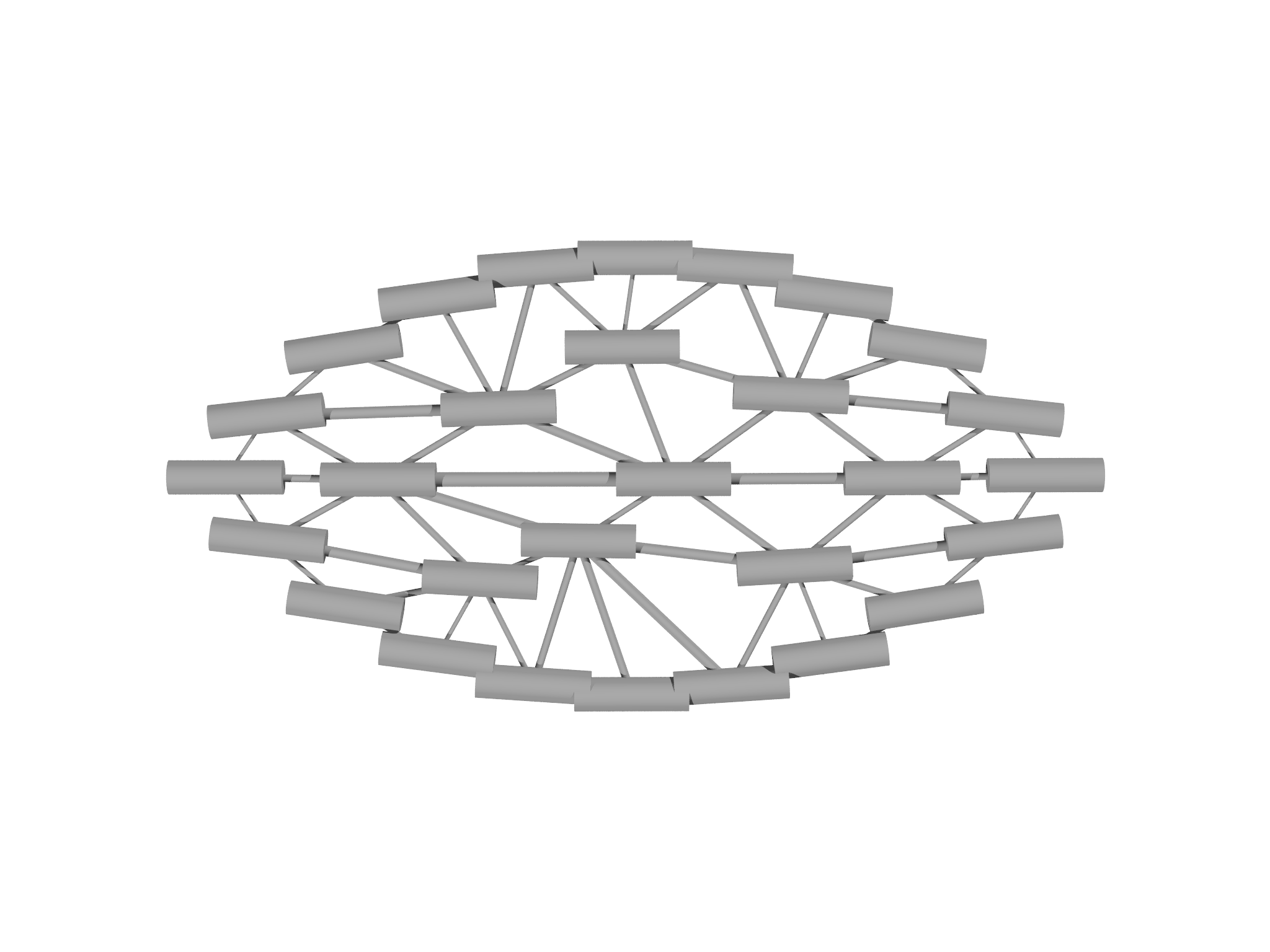
Next, we'll create a separate Graphics object that contains the director. Since the director \(\mathbf{n}\) is a unit vector field, and the sign is not significant (the nematic elastic energy is actually invariant under \(\mathbf{n}\to-\mathbf{n}\)), an appropriate way to display a single director is as a cylinder oriented along \(\mathbf{n}\). We will therefore make a helper function that creates a Graphics object and draws such a cylinder at every mesh point:

// Function to visualize a director field
// m - the mesh 
// nn - the director Field to visualize
// dl - scale the director 
fn visualize(m, nn, dl) { 
    var v = m.vertexmatrix()
    var nv = m.count() // Number of vertices
    var g = Graphics() // Create a graphics object
    for (i in 0...nv) {
    var x = v.column(i) // Get the ith vertex
    // Draw a cylinder aligned with nn at this vertex
    g.display(Cylinder(x-nn[i]*dl, x+nn[i]*dl, aspectratio=0.3))
    }
    return g
}

Once we've defined this function, we can use it:

var gnn=visualize(m, nn, 0.2)

The variables \(g\) and \(gnn\) now refer to two separate Graphics objects. We can combine them using the \(+\) operator, and display them like so:

var gdisp = g+gnn
Show(gdisp)

The resulting visualization is shown in Fig. 4.5.