Wrap

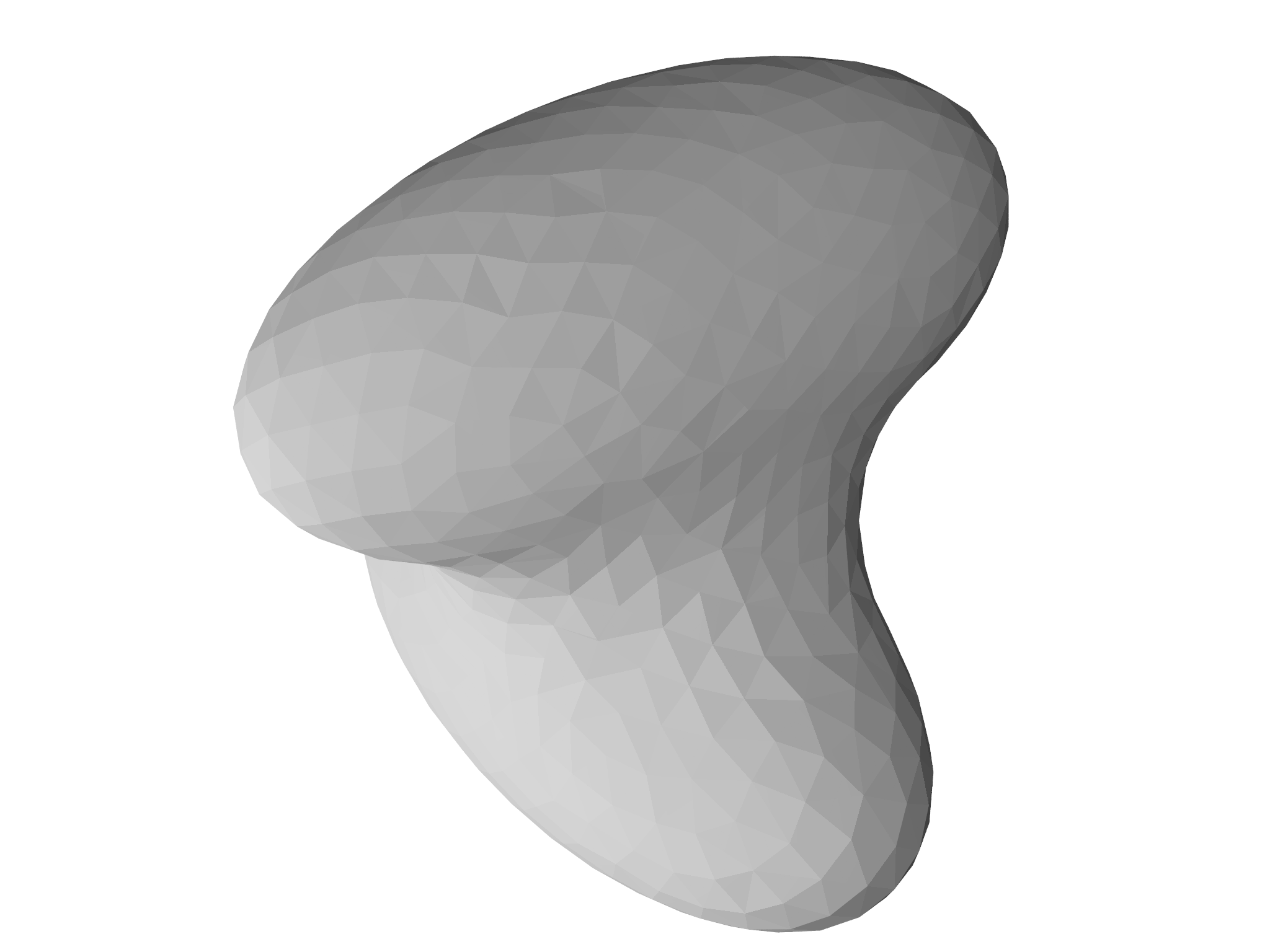
**Minimal surface constrained to lie outside two ellipsoidal one-sided level set constraints.**

The wrap example finds a minimal surface constrainted to lie outside two ellipsoids. The solution, shown in Fig. 7.13 could represent, for example, a possible configuration for a fluid bridge connecting two ellipsoidal particles.

The basic idea of this code is to "shrink wrap" the ellipsoids, starting with an initial mesh is a cube that completely encloses them. This is created with PolyhedronMesh from the meshtools module:

// Create a initial cube
var L = 2
var cube = [[-L, -L, -L], [-L, -L, L], [-L, L, -L],
            [-L, L, L], [L, -L, -L], [L, -L, L],
            [L, L, -L], [L, L, L]]

var faces = [[7, 3, 1, 5], [7, 5, 4, 6], [7, 6, 2, 3], [3, 2, 0, 1], [0, 2, 6,   4], [1, 0, 4, 5]]

var m=PolyhedronMesh(cube, faces)
m=refinemesh(m)

The particles are implemented as level set constraints. A convenient Ellipsoid class is defined to help create appropriate constraints,

class Ellipsoid { // Construct with Ellipsoid(origin, principalradii)
  init(x, r) { 
    self.origin = x
    self.principalradii = r
  }
  // Returns a level set function for this Ellipsoid
  levelset() {
    fn phi (x,y,z) {
      var x0 = self.origin, rr = self.principalradii
      return ((x-x0[0])/rr[0])^2 + ((y-x0[1])/rr[1])^2 + ((z-x0[2])/rr[2])^2 - 1     
    }
    return phi
  }
  /* Analogous code for gradient() ... */
}

The levelset method manufactures a scalar function representing the ellipsoid and suitable for use with the ScalarPotential functional. A second method, gradient, returns the gradient of that function.

The two ellipsoids of interest are then created like so:

var ell1 = Ellipsoid([0,1/2,0],[1/2,1/2,1])
var ell2 = Ellipsoid([0,-1/2,0],[1,1/2,1/2])

The optimization problem is set up to include the surface area subject to satisfaction of the level set constraints; these are noted as one-sided, i.e. satisfied if the mesh lies at any point outside the constraint region.

// We want to minimize the area
var la = Area() // Subject to level set constraints
var ls1 = ScalarPotential( ell1.levelset(), ell1.gradient() )
var ls2 = ScalarPotential( ell2.levelset(), ell2.gradient() )
var leq = EquiElement()

var problem = OptimizationProblem(m)
problem.addenergy(la)
problem.addlocalconstraint(ls1, onesided=true)
problem.addlocalconstraint(ls2, onesided=true)

To promote mesh quality, a second regularization problem is set up:

var reg = OptimizationProblem(m)
reg.addenergy(leq)
reg.addlocalconstraint(ls1, onesided=true)
reg.addlocalconstraint(ls2, onesided=true)

Optimization and refinement are performed iteratively:

sopt.stepsize=0.025
sopt.steplimit=0.1
ropt.stepsize=0.01
ropt.steplimit=0.2
for (refine in 1..3) {
  for (i in 1..100) {
    sopt.relax(5)
    ropt.conjugategradient(1)
    equiangulate(m)
  }
  var mr=MeshRefiner([m])
  var refmap = mr.refine()
  for (el in [problem, reg, sopt, ropt]) el.update(refmap)
  m = refmap[m]
}

Note that we set stepsize and steplimit on each optimizer; these values were found by trial and error. The initial shape is quite extreme, and so we use relax for the main optimization problem which is very robust. Calling equiangulate helps maintain mesh quality.