Qtensor
This example demonstrates use of the alternative Q-tensor formulation of nematic liquid crystal theory. We briefly present the necessary theory in two subsections below, then describe the implementation in morpho.
The Q tensor
In 2D, for a uniaxial nematic, we can define a Q-tensor: $$Q_{ij}=S(n_{i}n_{j}-1/2\delta_{ij})$$ Here, the \(-1/2\delta_{ij}\) is added for convenience, to make the matrix traceless: $$\text{Tr}(\mathbf{Q})=Q_{ii}=S(n_{i}n_{i}-1/2\delta_{ii})=S(1-1/2(2))=0$$ Now, the Q-tensor is also symmetric by definition: $$Q_{ij}=Q_{ji}$$ Due to these two reasons we can write the Q-tensor as a function of only \(Q_{xx}\) and \(Q_{xy}\):
$$ \mathbf{Q}= \begin{bmatrix} Q_{xx} & Q_{xy} \\ Q_{xy} & -Q_{xx} \end{bmatrix}. $$
Elastic Energy and Anchoring
The Landau-de Gennes equilibrium free energy for a nematic liquid crystal can be written in terms of the Q-tensor:
$$ F_{LDG}= \int_{\Omega}d^{2}{\bf x}\ \left(\frac{a_{2}}{2}\text{Tr}(\mathbf{Q}^{2})+\frac{a_{4}}{4}(\text{Tr}\mathbf{Q}^{2})^{2}+\frac{K}{2}(\nabla\mathbf{Q})^{2}\right) $$ $$ +\oint_{\partial\Omega}d{\bf x}\frac{1}{2}E_{A}\text{Tr}[(\mathbf{Q}-\mathbf{W})^{2}] $$
where \(a_{2}=(\rho-1)\) and \(a_{4}=(\rho+1)/\rho^{2}\) set the isotropic to nematic transition with \(\rho\) being the non-dimensional density. The system is in the isotropic state for \(\rho<1\) and in the nematic phase when \(\rho>1\). In the nematic phase, \(\ell_{n}=\sqrt{K/a_{2}}\) sets the nematic coherence length. Now,
$$\mathbf{Q}^{2}=\begin{bmatrix}Q_{xx} & Q_{xy} \\ Q_{xy} & -Q_{xx} \end{bmatrix}\begin{bmatrix}Q_{xx} & Q_{xy} \\ Q_{xy} & -Q_{xx} \end{bmatrix}=(Q_{xx}^{2}+Q_{xy}^{2})\begin{bmatrix}1 & 0 \\ 0 & 1 \end{bmatrix}$$ Hence, $$\text{Tr}(\mathbf{Q}^{2})=2(Q_{xx}^{2}+Q_{xy}^{2})$$ Similarly, $$(\nabla\mathbf{Q})^{2}=\partial_{i}Q_{kj}\partial_{i}Q_{kj}=2{(\partial_{x}Q_{xx})^{2}+(\partial_{x}Q_{xy})^{2}+(\partial_{y}Q_{xx})^{2}+(\partial_{y}Q_{xy})^{2}}$$ Now, the second term is a boundary integral, with \(E_{A}\) being the anchoring strength. \(\mathbf{W}\) is the tensor corresponding to the boundary condition. For instance, for parallel anchoring, $$W_{ij}=(t_{i}t_{j}-1/2\delta_{ij})$$ where \(t_{i}\) is a component of the tangent vector at the boundary. \(\mathbf{W}\) is also a symmetric traceless tensor with two independent components \(W_{xx}\) and \(W_{xy}\). The boundary term becomes: $$\text{Tr}[(\mathbf{Q}-\mathbf{W})^{2}]=2{Q_{xx}^{2}+Q_{xy}^{2}-2(Q_{xx}W_{xx}+Q_{xy}W_{xy})+W_{xx}^{2}+W_{xy}^{2}}$$
Optimization problem
We can formulate all the preceding expressions in terms of vector quantities: $$\vec{q}\equiv \{ Q_{xx},Q_{xy} \} $$ $$\vec{w}\equiv \{w_{xx},w_{xy} \}$$ Thus, $$\text{Tr}(\mathbf{Q}^{2})=2||\vec{q}||^{2}$$
$$(\nabla\mathbf{Q})^{2}=2||\nabla\vec{q}||^{2}$$
$$\text{Tr}[(\mathbf{Q}-\mathbf{W})^{2}]=2||\vec{q}-\vec{w}||^{2}$$ With these, we want to minimize the area-integral of $$F=\int_{\Omega}d^{2}{\bf x}\ \left(a_{2}||\vec{q}||^{2}+a_{4}||\vec{q}||^{4}+K||\nabla\vec{q}||^{2}\right)$$ together with the line-integral energy $$\oint_{\partial\Omega}d{\bf x}\ E_{A}||\vec{q}-\vec{w}||^{2}$$
Implementation
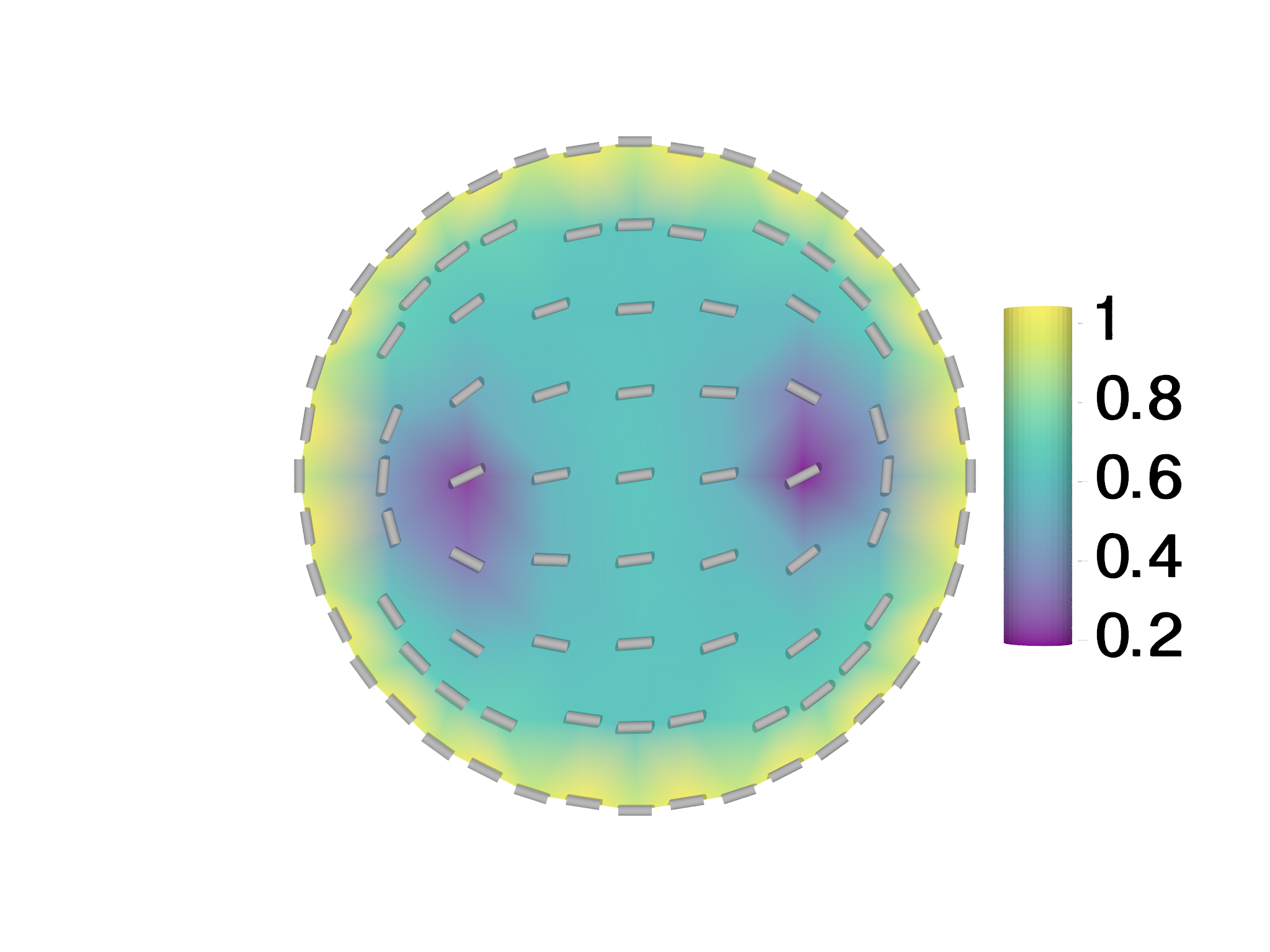
This free energy is readily set up in morpho. For this example, we consider a 2D disk geometry with unit radius. We use \(\rho=1.3\), so that we are deep in the nematic regime. We fix \(E_{\text{A}}=3\), which sets strong anchoring at the boundary. With this strong tangential anchoring, we get a topological charge of \(+1\) at the boundary, and this acts as a constraint. When the nematic coherence length is comparable to the disk diameter (\(\ell_{n}\sim R\)), the \(+1\) charge penetrates throughout the disk, whereas if (\(\ell_{n}\ll R\)), then a formation with 2 \(+1/2\) defects is more stable. To test this, we use two different values of \(K\):, 0.01 and 1.0.
We first define all our parameters and import \(\texttt{disk.mesh}\) from the tactoid example:
var rho = 1.3 // Deep in the nematic phase
var EA = 3 // Anchoring strength
var K = 0.01 // Bending modulus

var a2 = (1-rho)
var a4 = (1+rho)/rho^2

var m = Mesh("disk.mesh")
var m = refinemesh(m) // Refining for a better result
var bnd = Selection(m, boundary=true)
bnd.addgrade(0) // add point elements
We define the Q-tensor in its vector form as discussed above, initializing it to small random values:
var q_tensor = Field(m, fn(x,y,z)
Matrix([0.01*random(1), 0.01*random(1)]))
Note that this incidentally makes the director parallel to a 45 degree line. We now define the bulk energy, the anchoring energy and the distortion free energy as follows:
// Define bulk free energy
fn landau(x, q) {
  var qt = q.norm()
  var qt2=qt*qt
  return a2*qt2 + a4*qt2*qt2
}
// Define anchoring energy at the boundary
fn anchoring(x, q) {
  var t = tangent()
  var wxx = t[0]*t[0]-0.5
  var wxy = t[0]*t[1]
  return (q[0]-wxx)^2+(q[1]-wxy)^2
}

var bulk = AreaIntegral(landau, q_tensor)
var anchor = LineIntegral(anchoring, q_tensor)
var elastic = GradSq(q_tensor)
Equipped with the energies, we define the OptimizationProblem:
var problem = OptimizationProblem(m)
problem.addenergy(bulk)
problem.addenergy(elastic, prefactor = K)
problem.addenergy(anchor, selection=bnd, prefactor=EA)
To minimize the energy with respect to the field, we define the
FieldOptimizer and perform a linesearch:
var opt = FieldOptimizer(problem, q_tensor)
opt.linesearch(500)
Visualization
For visualizing the final configuration, we use the same piece of code we used for the tactoid example, and define some additional helper functions to extract the director and the order from the Q-tensor:
fn qtodirector(q) {
  var S = 2*q.norm()
  var Q = q/S
  var nx = sqrt(Q[0]+0.5)
  var ny = abs(Q[1]/nx)
  nx*=sign(Q[1])
  return Matrix([nx,ny,0])
}

fn qtoorder(q) {
  var S = 2*q.norm()
  return S
}
We use these to create Fields from q_tensor.
// Convert the q-tensor to the director and order
var nn = Field(m, Matrix([1,0,0]))
for (i in 0...m.count()) nn[i]=qtodirector(q_tensor[i])
var S = Field(m, 0)
for (i in 0...m.count()) S[i]=qtoorder(q_tensor[i])
and display these, reusing the visualize function from the tactoid
tutorial example.
var splot = plotfield(S, style="interpolate")
var gnn=visualize(m, nn, 0.05)
var gdisp = splot+gnn
Show(gdisp)
This creates beautiful plots of the nematic, displayed in Fig. 7.11. Like the tactoid example, we can do adaptive mesh refinement based on the elastic energy density as well.