Morpho Manual

DLA

Diffusion Limited Aggregation is a process describing the formation of aggregates of sticky particles. An initial seed particle of radius \(r\) is placed at \( x_0=(0,0,0) \). Subsequent particles are added one by one from initial random points \(\mathbf{x}_{i}^{0}=R\mathbf{\xi}/|\mathbf{\xi}|\) where \(\xi\) is a random point normally distributed in each axis; the construction \(\mathbf{\xi}/|\mathbf{\xi}|\) generates a random point on the unit sphere. In morpho, this looks like

fn randompt() {
  var x = Matrix([randomnormal(), randomnormal(), randomnormal()])
  return R*x/x.norm() 
}

The mobile particle moves diffusively, according to

$$ x_i^{n+1}=x_i^{n}+\delta\xi$$

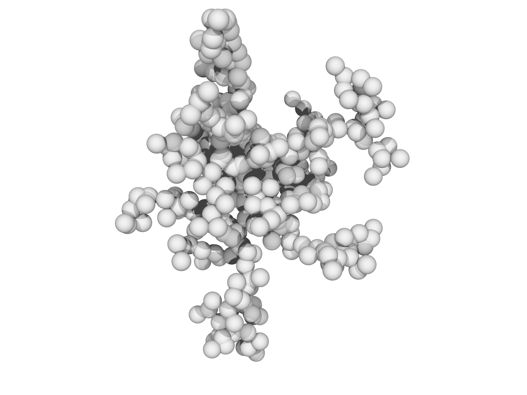
where \(\delta\) is a small number. As the particle moves, we check to see if it has collided with any other particles, $$\left|x_{i}-x_{j}\right|<2r,\forall i\neq j,\label{eq:collisioncheck}$$ or if it has wandered out of bounds, $$\left|x_{i}\right|>2R.$$ If a particle has collided with another particle, it becomes fixed in place and joins the aggregate. As particles are added, the aggregate develops a characteristic fractalline morphology as shown in Fig. 7.5{reference-type="ref" reference="fig:DLA"}. The body of the program is a double loop:

for (n in 1..Np) { // Add particles one-by-one  
  var x = randompt()
  while (true) {
    // Move current particle
    x+=Matrix([delta*randomnormal(), delta*randomnormal(), delta*randomnormal()])

    // Check for collisions
    /* ... */

    // Catch if it wandered out of the boundary
    if (x.norm()>2*R) x = randompt() 
  }
}

To perform the collision check, the example uses a data structure called a \(k\)-dimensional tree, provided in the kdtree module. A \(k\)-dimensional tree provides a nearest neighbor search with \(O(\log N)\) complexity rather than \(O(N)\) complexity as would be required by searching all the points directly. The collision check code looks like this:

if ((tree.nearest(x).location-x).norm()<2*r) {
  tree.insert(x)
  pts.append(x)
  if (x.norm()>R/2) R = 2*x.norm()
  break // Move to next particle
}

Notice that we gradually expand \(R\) as the aggregate grows. Ideally, each point should start very far away, really at infinity, but this would be very expensive in terms of the number of diffusion steps. A value of \(R\) double the greatest extent of the aggregate is a good compromise between speed and a reasonable approximation of diffusion limited aggregation.

This example also demonstrates how to create a simple custom visualization directly using the graphics module. The particles are drawn as spheres and displayed with the following code. An example run is displayed in Fig. 7.5.

var col = Gray(0.5)
var g = Graphics()
g.background = White
for (x in pts) g.display(Sphere(x, r, color=col))
Show(g)